A downloadable pdf version is available: [ 📄 here ]
Alexander Gusev
A word on not being an easy mark
A word on basic moral principles
1.2 | Genetics, Environment, Interactions, and Assortment
2.5 | Population stratification
2.6 | A word on “molecular” kinship heritability
2.7 | Putting it together: environmental confounding in genetic studies
2.8 | Functional partitioning of h2g
2.9 | Biases due to cross trait assortative mating
Direct and indirect heritability
3.3 | Estimation bias due to assortative mating
3.4 | Interpretation of direct heritability and indirect associations
3.5 | Biases in population heritability under AM and VCT
3.6 | A word on ongoing challenges for within-family analyses
The genetic architecture of common traits
4.1 | Common variant population h2g
4.3 | Heritability explained by environmental confounding/rGE
4.4 | Natural selection and expectations for rare variants
4.5 | Low-frequency variant h2g partitioning
4.8 | A word on heritability in animals
The heritability of educational attainment
5.3 | Common direct heritability and PGIs
5.4 | Common population heritability (with environmental confounding)
5.5 | Measurable environmental confounding in population PGIs
5.6 | Interpreting h2g parameters under a cultural transmission model
5.7 | Gene-Environment interactions / Scarr-Rowe
5.8 | Direct common effects on other phenotypes
5.9 | Functional interpretation of common variant h2g
5.10 | Rare variant heritability and gene-level analyses
5.11 | A word on adoption studies
5.13 | A word on “natural selection” using EA PGIs
5.14 | A word on latent assortment
5.15 | A word on EA PGI accuracy
5.16 | A few words on scientific value and responsibility
The heritability of IQ test performance I: What does IQ measure?
6.1 | Premise: What are IQ tests and what are they good for?
6.3 | Theories of the positive manifold
6.4 | The measurement of IQ and five paradoxes
6.5 | Empirical evidence for theories of the positive manifold
8.0 | Read these books instead!
8.5 | Selection with drift and “effective neutrality”
8.6 | Linked and background selection (BGS)
8.7 | Differentiation within/between populations / FST
8.8 | Complex trait differentiation / Qst
8.10 | Testing for locus-specific selection
8.11 | The Breeder’s Equation and heritability (revisited)
Concepts: race and genetic ancestry
9.1 | Definitions and conceptual models of race
9.2 | Race provides a poor fit to genetic variation
9.4 | Continuous ancestry / Principal Components Analysis (PCA)
9.5 | A word on nonlinear dimensionality reduction / UMAP
9.6 | Model-based clustering of ancestry / STRUCTURE
9.7 | A word on parametric models / admixture graphs
9.8 | A final word on ancestry “realism”
9.9 | Genetic ancestry in real data
9.10 | Human history through the lens of modern and ancient DNA
When ordinary people talk to geneticists, the questions they often most want to have answered are: “How much does genetics matter for behavior?” and “Is race real?”. These will sometimes fold together to form a third question: “Are racial differences in behavior and outcomes explained by genetics?”. Contrary to popular belief, all three questions have been heavily debated for decades within the fields of quantitative, population, and behavioral genetics. In many cases these questions are unanswerable or ill-posed, but the field has expanded great effort into understanding why they are unanswerable, what one can expect from theory, and what is answerable with data. Millions of individuals have been genotyped to answer questions like “how much of your educational attainment is in your genes?” or “how do the effects of genetic variants differ across populations?”. However, many of these discussions happen behind journal paywalls or in single sentence news quotes and do not filter down in a coherent way to the general public. The goal of this document is to distill the recent findings from molecular studies of behavioral traits and group differences in a way that is both comprehensive and broadly understandable. In the end, my hope is that the lay reader has the tools and general understanding to seek out accurate answers to the complicated questions in genetics. For readers with expertise in genetics, my hope is that this document will tie together concepts that still typically reside in individual papers and supplementary notes into a bigger whole and identify important limitations and open questions.
Molecular data (i.e. directly measured genetic variation) provides opportunities to use the subtle variations between individuals and groups to better distinguish correlation from causation. When we know who has which genetic variant we can: look at unrelated individuals that are unlikely to directly share environments and ask if subtle differences in their genetic variability relate to their phenotype; look at siblings and quantify if subtle differences in the specific alleles they share relate to their outcomes; use genetic data from students who experienced some intervention – say, staying in school for an extra year – and ask if subtle genetic differences in them or their families influenced the effectiveness of the intervention; etc and so on. Having tools to distinguish correlations (patterns that we tend to observe in the world) from causes (factors that influence changes in the world) is critical to understanding how our world and society works and has been greatly enabled by molecular studies (R. C. Lewontin 2006).
Molecular genetics is also simply becoming a bigger part of life. Ordinary people are often experiencing genetics through commercial services quantifying cancer risk genes, polygenic scores, and genetic ancestry. There is a need for context and clarity on what these molecular tools can and cannot tell us.
Large-scale genetic studies present a genuine opportunity to expand our understanding of the world. But they also involve the use of complicated statistical techniques, large datasets that often can’t be manually inspected, and opaque quantities. Naturally, this has created space for scammers and bigots who can exploit the complexity of data. Just as it is important to distinguish correlations from causes, it is important not to be an easy mark for con artists. Spend some time discussing these questions out in the world and you will run into several common trends: (a) misrepresentation of what is being estimated: not defining (or defining imprecisely) the quantities of interest; (b) misrepresentation of causal versus correlational studies, and particularly a preference for broad claims from correlative studies over precise claims from causal studies; (c) the gish gallop: jumping from topic to topic or study to study rather than attempting to reach an understanding (often making use of [a] and [b] along the way). This document will thus strive to (a) provide precise definitions, (b) distinguish correlation/causation, and (c) present findings comprehensively. In later sections, some time will also be spent discussing common scams and misconceptions.
There is no question as to the moral dignity and respect for all individuals. It is wrong to treat people differently simply because they belong to a certain race/ethnicity, sex/gender/sexual orientation, national origin, or religion. It is wrong to allow harm to people for factors they have little or no control over. A fundamental principle of our society is that individuals have a right to be treated as individuals and this principle does not hinge on parameters of heritability, group variance, or group mean.
Genetic findings often still take on a moral valence with respect to how one should feel about unfairness in the world and how much can be done to change it. And let’s be honest: many people just want to use genetics as an excuse to see the current (or prior) state of society as “the way things are meant to be” or to be cruel to others. As heritability is a descriptive, non-causal, mathematical abstraction (see below) it provides no insights on moral questions. Anyone using genetics to argue against moral dignity or claim that genetics tells us how things “should be” is taking you for an easy mark.
The definition of heritability has been discussed and debated for decades, often starting from assumptions on genetic causality, independence of environments, and selective breeding and then working backwards to caveats and limitations in real populations (Stoltenberg 1997). In plants, cattle, or dogs (where the terminology originated) assumptions about environments and selective breeding may be reasonable or directly testable and modifiable. In humans, the genetics/environment dichotomy does not hold and so a causal definition is either erroneous from the start or unusably vague. Here, I will instead define heritability in purely correlative/predictive terms and then work forwards to the very limited set of causal conclusions we can draw from it.
Let’s start simple and build up. Consider a continuous trait [y] that varies in a given population and a single genetic variant [x]: the “heritability” of that variant is the magnitude of its association with the trait, or the squared correlation between [x] and [y]. Run a large genetic study, correlate [x] and [y], square the correlation (and adjust for noise), and you have the heritability of that trait attributable to that variant – that’s it! Note that we’ve made no assumptions about how [x] associates with [y]: it could be causally impacting the trait in the individual or non-causally correlated with some environment that influenced their trait (or a technical artifact for that matter): all heritability quantifies is the magnitude of the correlation.
For “complex” traits, where many genetic mutations are associated, each with some positive or negative “effect size”, the genetic value of that trait in an individual is the sum of all the increasing/decreasing effects they carry. If we then think of the total trait as a simple sum of the genetic value and an independent environmental value, the additive heritability is the ratio of the variance of the genetic value over the total variance. When heritability is 0, that means the variance of the trait cannot be assigned to any of the genetic value, and when heritability is 1 that means the variance of the trait can be assigned to all of the genetic value. I’m using the terms “can/cannot be assigned” because we’ve made the simplifying assumption that the genetic and environmental terms are independent. In the real world, genetics and environment are obviously not independent “components” but correlated and interacting processes; every estimator of heritability implicitly or explicitly makes a choice about how to assign the correlated variance. Since an oracle will not tell us which assignment is correct, heritability (and related terms like “genetic values”) is thus always an abstraction of complex underlying processes (more on this later).
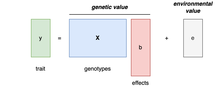
Mathematically, that additive model looks like this:
Heritability is Var(Xb)/Var(y) or equivalently the squared correlation between the genetic value and the trait [Cor(Xb,y)^2], where [Xb] is also the best additive genetic predictor of [y]. This is perhaps the most direct definition of heritability: how much of [y] could have been predicted from a weighted sum of [X]. This definition is specific to the population in which it is being estimated and to the genetic variation that goes into estimating it.
Finally, a bit of jargon: heritability from the additive model is also often called “narrow sense” heritability, in contrast to “broad-sense” heritability which also includes the contribution of non-additive (e.g. dominance) and interaction effects. At the molecular level, the distinction between additive and non-additive terms is somewhat arbitrary, since one can include non-additive combinations of genetic material in [X] (for example, [X] could be defined to contain all pairs of [xi*xj] mutation products and thus also estimate the association of two-way interactions or all [xi2] terms to estimate dominance).
Heritability is not a causal parameter. Because genotypes precede phenotypes and (generally) cannot be influenced by phenotypes, heritability is often implicitly treated as being causal when it is not. As a simple example, if you have two variants ([xC] and [xNC]) that are perfectly correlated in the population and [xC] influences the trait while the [xNC] doesn’t (i.e. it is a “tag”), the heritability from [xNC] alone will be the same as the heritability from [xC] alone (and will be the same as the heritability from [xC,xNC] together). This is important because if we intervene on [xNC] we will not actually influence the trait. Disentangling causality gets more complicated if, for example, genetic variants in a study participant are correlated with genetic variants in their parents, who also influenced their trait through the environment: now this variation is completely non-causal in the participant and, in fact, should point us to interventions on the parenting environment rather than on a genetic mechanism.
The fact that heritability feels intuitively causal but is merely a correlation makes it ripe for misinformation. Where ordinarily it would be nonsensical to argue that just because we see that two populations have different rates of college attainment we therefore know what causes the difference; a bullshit artist can invoke the “high heritability of education” (perhaps even rattle off a few twin study estimates to the decimal point) and claim confidently that the cause must be “bad genes”, cloaked in the appearance of scientific rigor. This has created a cottage industry of “noticers”, who loudly “notice” that certain demographics are associated with certain outcomes and either explicitly or implicitly argue that, since those outcomes are heritable, these correlations must also be causal and deterministic. Causal inference is hard but “noticing” is easy, and so noticers can stay busy spotting meaningless correlations, hoping that you will be convinced by the sheer volume of their observations.
Heritability does not tell us anything about the malleability of a trait (i.e. whether the trait can be intervened on or modified). Even when all of the assumptions are met and the estimates are unbiased, heritability is just a quantification of the association of genetics and environment with the trait; changing the environment can make the genetics irrelevant or changing the genetics could make the environment irrelevant. Consider the classic example of eyesight: highly heritable but easily malleable through the use of glasses (high heritability, high malleability). Are glasses a “large” environmental variance that’s compensating for high heritability? The question is clearly nonsensical: variance is a mathematical concept and the mathematical variance of glasses-wearing trivially depends on how many people have them. But this is the kind of logic one gets into when thinking that heritability is a surrogate for malleability. For an example in the opposite direction, consider the case of the gene PCSK9: a tiny number of individuals carry rare loss-of-function mutations in PCSK9 that dramatically reduce their bad cholesterol, but because most people carry a normal functioning version of PCSK9, these variants do not “explain” much of the population variance in bad cholesterol (i.e. contribute much to heritability). However, when drugs that inhibit PCSK9 are administered to the general population they have a highly significant effect on the trait mean (low heritability, high malleability).
Other historical examples include the rapid change in human height over the past 100 years or the rapid growth in educational attainment in the US. Height has changed rankings across continental groups, almost certainly brought on by improved nutrition. Even though it is a highly heritable trait (by nearly any estimate), mean height has shifted by ~2 standard deviations in just five generations (insufficient time for any evolution to have occurred). But ask most people and they will tell you height is just the way it is because of genetics. Significant increases in height have even been observed within western countries in the past several generations (Fredriks et al. 2000). Likewise, there has been rapid growth in educational attainment in the US. The number of college graduates has doubled from 1980 to today (notably, the former would be the time a typical contemporary biobank participant was of college-age). Are these changes driven by low heritability? Almost certainly not, heritability is merely a retrospective measure and does not tell us about the prospective impact of changing the environment.
Substantial changes in educational attainment in the US and height globally/nationally.
(left) Changes in the percentage of the US population who have completed high-school or college over time; (middle) Changes in adult male height over a century; (right) changes in height in The Netherlands from 1955 to 1997, attributed to improved nutrition, health, and hygiene.
Heritability does not tell us anything about a population mean/average, because it operates on variance. For example, if everyone in a given population suddenly grew exactly 5 inches, the heritability of height would stay the same because only the population mean (and not the variance) will have changed. In fact, it is quite common in heritability analyses to center and scale the trait and regress out nuisance covariates so that the heritability estimate loses any “real world” scale entirely.
Heritability does not tell us anything about the total variance of the trait, because it is just a proportion of the total variance. Imagine a future where a drug eradicates some disease, except for a small number of people who cannot tolerate the drug because of a pathogenic mutation. In this society, the heritability of the disease is now 100% – all disease cases are caused by a genetic mutation – but the variance of the disease is very low. In contrast, most adults have two eyes except for those who experience an environmental trauma – the variance is low and the heritability is low. So the notions of heritability, mean, and variance are distinct.
To illustrate these points, let’s look at very different traits that produce the same heritability (i.e. the correlation of the genetic component and the total trait is 50% in the population). It’s trivial to see that shifts in mean have no effect on the heritability estimate and neither do compensatory shifts in variance (i.e. when both genetic variance and trait variance are shrunk). One can additionally construct more complex scenarios with subgroup heterogeneity or Gene-Environment interaction that produce equivalent heritability estimates by simply fiddling with various variance terms. In short, heritability tells us how much of the trait could have been predicted from the genetics in the population we studied, with no guarantees on causality, malleability, or trait architecture.
Six very different traits with equivalent heritabilities.
The distribution of the genetic value (pink), environmental value (green), and total trait (black) is shown for: (a) A trait with 50% genetic variance and 50% environmental variance; (b) A trait where the genetic value has been shifted by five standard deviations; (c) A trait where the environmental value has been shifted by five standard deviations; (d) A trait with 25% genetic variance and 25% environmental variance; (e) A trait with two subpopulations, one of which has a genetic value shifted by two standard deviations and environmental variance increased by five-fold; (f) A trait with 50% genetic variance, 5% environmental variance and 45% gene-environment interaction variance. In all six instances, the squared correlation between the genetic value and the phenotype is 0.5
Up to this point we’ve considered heritability for continuous traits, where [Xb] ads up to a numerical value (e.g. height). For dichotomous (aka case/control) traits, this formulation is modified slightly so that [y] is an underlying normally distributed liability, and individuals who exceed a threshold of liability are affected/cases while the rest are controls. In other words, a transformation is applied to [y] to turn the top x% into cases, where x is the disease prevalence. This is the liability threshold model and it is the primary statistical model for working with dichotomous traits.
The figure below shows various consequences of this transformation as a function of h2g and disease prevalence. There are several details to notice. First, the amount of genetic variation within families is surprisingly high: even for a trait with heritability of 100% and a prevalence of 40%, the risk for an individual increases to just ~60% if they have an affected relative or 80% with two affected parents. This means that even for a completely heritable trait, there will be many families in which both parents are cases and the child is not. Second, individual risk depends on both the heritability and the prevalence. So for a trait with heritability of 100% and a prevalence of 1%, the risk for an individual with an affected sibling is still just ~15% – this is much higher than the population prevalence but still much lower than heritability alone might imply. Third, classification accuracy (defined as Area Under the Curve for a binary predictor based on the genetic value) is highly non-linear with respect to the heritability especially for low prevalence traits. It is thus difficult to think intuitively about how heritability translates into the ability to distinguish cases from controls.
Aspects of the liability threshold model.
(left) Classification accuracy, (middle) the probability that an individual is an affected case given their sibling is a case, (right) the risk that an individual is an affected case given both their parents are cases. In each plot, the results are shown for three levels of prevalence and points are indicated for representative heritabilities: 5% (roughly the h2g of educational attainment), 20% (roughly the h2g of hypertension and other biomarker traits), 80% (roughly the twin h2 of height and other highly heritable traits).
The discussion about heritability often touches on the “missing heritability” question. Generally speaking, “missing heritability” can be thought of as a significant discrepancy between different estimators of heritability. Some people use “missing heritability” to refer to the discrepancy between twin-based and molecular-based estimates. Some people use “missing heritability” to refer to the discrepancy between what can be explained by individual, known mutations (i.e. significant associations from a GWAS) and the total molecular-based estimate across all mutations (regardless of significance). Most of the time the term only adds confusion and obfuscates the fact that different methods are estimating different parameters. It also implicitly presumes that the missing heritability could be “found”, which of course is not certain (for example if one estimate is simply biased upwards).
In the real world, traits are not just the sum of a genetic value and an independent environmental value, they are a function of many complex relationships. To develop an understanding of these relationships, we typically break them down into further components of the trait variance. These components are important to define precisely because they are often assigned, estimated, or ignored differently by different models. Most of the time, models set certain components to zero or try to quantify what can be assigned to additive genetics and then what is left. In the cartoon below, a perfect interaction between two terms would result in assigning all of the variance in outcome to one term or the other arbitrarily. Indeed, complex relationships between genetics and environment can even yield significantly negative estimates of heritability, which no longer have a plausible interpretation as squared correlations but can be entirely statistically valid as models of trait covariance (Steinsaltz, Dahl, and Wachter 2020).
Cartoon thought experiment of additive versus interactive models.
(left) The trait is an abstract sum of an independent genetic and environmental component. (right) The trait is a more plausible interaction between a genetic and an environmental component. With interactions, the partitioning of variance into additive genetic and environmental terms (i.e. “nature” and “nurture”) is not singularly defined and assumptions/constraints have to be made on how to partition/assign the contribution from “Billy” or “Suzy”. Figure from (Moore and Shenk 2017).
GxG (or “epistasis”) refers to the non-additive combined effects of a single or multiple causal variants. For example, a recessive effect – where a variant only impacts the trait when both hazardous alleles are present – can be thought of as a single-variant interaction. If the alleles at two different variants need to be the same for an effect on the trait, this is a two-variant (or second order) interaction, and so on for higher order interactions.
Schematic of single-locus GxG (recessive), multi-locus GxG (epistasis), and GxE.
Blue squares indicate genetic/environmental contexts and yellow/orange/red squares indicate a low/medium/high effect on the trait for that context combination. Note that in all three examples, much of the non-additive effect can still be “tagged” by an additive model but will be dampened relative to the true interaction model. A/T are the alleles of one variant; G/C are the alleles of a second variant; and E1/E1 are two environments.
GxE refers to the interaction between genotype and environment on the trait. For example, if a mutation only has an effect on the trait in smokers and not non-smokers, this is a GxE interaction where the E (environment) is smoking. Note that E can refer to essentially any non-genetic factor/exposure. A challenge for heritability estimation is where to assign the contribution of GxE since both factors need to be in play for the effect to manifest itself; this then becomes a modeling decision that leads to differences across different estimators.
In addition to the simple model where a mutation has an effect in one context and not another, a more subtle “amplification” model of GxE has been proposed. Under amplification, the genetic effects between two environments are correlated but differ by some magnitude (for example, the effects of all/many alleles in older participants are 1.2x higher in magnitude than the effects in younger participants). This form of GxE would produce high genetic correlations but large differences in heritability between environments.
It’s important to distinguish between mechanistic interactions – non-additive effects between two mechanisms in the underlying causal model, and statistical interactions – significant interaction terms in an inferential model. Different ways of processing data can mask a true mechanistic interaction or induce a false statistical interaction. In general, this happens when the “scale” or “functional form” of the response variable is either unknown or distorted by data processing.
For example, let’s generate data with a true multiplicative interaction ([y = x*z]) where [x] is a continuous variable and [z] is a binary group. When we fit a standard linear model to this data ([y ~ x + z + x*z]) the interaction term is highly statistically significant. Since we have two groups here, an interaction model is equivalent to testing for a difference in slope between them, and when we plot the two groups (below) we can indeed see a significant difference in slope. If we instead log transform the data first, a very common practice to “stabilize” features with high variance, we have turned the outcome into [y = x + z] and the linear model no longer identifies an interaction. Moreover, the transformed data actually produces a better fit to the features, so a “data-driven” analysis would tell us that the transformation is more parsimonious and no interaction is present.
Data transformation masks a true mechanistic interaction.
On the left, the true generative process for a continuous variable interacting with a binary group (purple/black). On the right, the same data is log transformed and the true interaction disappears (and the fit improves).
Now let’s consider the opposite effect. We first generate data without an interaction ([y = x + z]) and fit a standard linear model. As expected, the slopes are the same in the two groups and no interaction is identified. Next, we dichotomize the data based on an arbitrary cutoff; let’s say individuals above a certain value of [x] are cases and the rest are controls. In a linear model, the slope in each group will depend on the fraction of cases in that group, so if one group has many fewer cases (for example, they are systematically healthier but the influence of [x] is the same) the effect of [x] will appear weaker. In a linear model, this yields a significant statistical interaction term. Statistical interactions become even more complicated to interpret for ordinal, count-based, or survival processes (Domingue et al. 2020).
Analysis of a binary variable with a linear model induces a statistical intearction.
On the left, a generative process for two groups (purple/black) with no interaction with the continuous variable (x-axis). On the right, the continuous variable is transformed into a binary variable based on a threshold (dashed line in the left plot) that produces case imbalance. This induces a significant interaction between the variable and the group.
In short, a statistical interaction is neither necessary nor sufficient evidence of an underlying mechanistic interaction. Statistical interactions can still be useful for modeling; for example by improving predictive accuracy, adjusting for undesirable artifacts, or evaluating counterfactuals/interventions (Thompson 1991). But additional mechanistic evidence is needed for a causal interpretation; goodness of fit alone is not enough. Data that are highly non-linear or exhibit strong class imbalance are particularly sensitive to modeling assumptions.
rGE refers to correlations between genetics and environment which may or may not be caused by genetics. An example I will refer to frequently is a genetic variant that causes allergies, which nudges people to move from rural to urban areas. In a rural parent, this variant has a direct causal effect on the trait. In their urban off-spring, this variant will now be correlated with everything else they experience in that urban setting. Even generations later when allergies have been cured, the allele may still be slightly elevated in – and thus correlated – with the urban environment. This example may seem far-fetched, but in a biobank of half a million individuals such subtle changes are detectable, and in fact just such an allergy variant was recently identified and associated with geography (rs5743618, one of the strongest associations with hayfever) (Hu et al. 2023). Another example is that of genetic variants that influence parental behavior (for example, variants that are associated with postpartum depression). In parents, the variants influence the environment for their children. When passed down to those children, the variants will be correlated with the trait consequences of that environment, even though it is no longer playing a causal role in the child. These are both examples of “passive rGE”. Various cultural structures can substantially amplify passive rGE associations well beyond their true underlying causal effect (see [3]).
An “active rGE” correlation can arise when genetic variation causes individuals to enter specific environments that alter their trait. For example, a variant that nudges carriers to be more outgoing, which places them in more social situations, which further reinforces their outgoing or sociable nature, and so on. In this case, the genetic variant may initially appear to have little association with the environment, but a causal association increases over time. Finally, when variants lead to behavior in children that then elicit certain behaviors and environments from their parents/relatives (who also share genetic variation with them), this creates a feed-back loop known as “evocative rGE”. Of course, individuals who carry the variant but are not able to participate in the relevant environment will not exhibit this rGE. As with GxE, the assignment of rGE is another modeling decision that can lead to differences across different estimators.
Forms of rGE: Passive, Evocative, and Active Gene-Environment correlation.
Blue indicates causal factors; green indicates outcomes; red and dashed lines indicate non-causal factors and relationships. Bi-directional arrows reflect interactions or reciprocal effects. Adapted from (Avinun 2020)
Assortative mating (also referred to as “homogamy”) is a social process where partners/mates pair up based on observed or latent phenotypes (e.g. “tall people like to marry tall people”). Assortment on heritable traits is common, with the highest AM typically observed for educational attainment and other/related behavioral phenotypes. Notably, AM on educational attainment (0.48) and political values (>0.5) is higher than AM on IQ (0.23) (Horwitz et al. 2023), reiterating that AM is a social process and class signifiers can have higher AM than latent traits. AM on a heritable phenotype will influence the apparent genetic variance in offspring/family studies (i.e. siblings will be more genetically similar than expected because their parents are more genetically similar than expected) as well as the correlation between trait influencing alleles (Crow and Felsenstein 1968; Loïc Yengo et al. 2018). AM thus further complicates the interpretation of heritability: the same exact variants and causal effects in the same exact environment will produce different values of genetic variance (and thus heritability) under different mating patterns. In particular, the association of genetic variance with the trait (i.e. the true [Cor(Xb,y)^2] is higher under AM than it would be with the same genetics and environment under random mating (more on this later).
When AM is constant over time, it induces correlations with each generation, roughly half of which are observed within the first generation and typically reaching “equilibrium” within five generations. Methods that account for AM typically assume that equilibrium has been reached to simplify their derivations. Lack of equilibrium (i.e. steadily increasing or decreasing AM) would cause an estimate not to generalize beyond the estimated generation.
Impact of heritability and assortative mating on correlations at putatively independent markers.
Assortative mating on a heritable phenotype leads to a sudden increase in the correlation of causal alleles in the population, which stabilizes at an “equilibrium” in ~5 generations. The correlation increases with higher heritability or stronger assortment. Simulations using 10 markers and 10,000 individuals.
A related concept is cross-trait AM (xAM), where mates pair up based on matching on different traits (for example, educated women preferentially pair up with tall men) (Border, Athanasiadis, et al. 2022). xAM will cause genetic variants influencing a trait in one partner to be correlated with variants influencing a different trait in another, and may also create apparent genetic correlations in population studies.
Genetic correlation is an estimate of the sharing of genetic variance across pairs of traits (van Rheenen et al. 2019). Formally, for two traits {y1,y2} with causal effect sizes {b1,b2}, genetic correlation can be thought of as Cov(X’b1,X’b2)/sqrt(Var(X’b1)Var(X’b2)), where Cov(X’b1,X’b2) is the genetic covariance between the traits. This is equivalent to the correlation of the genetic values [Cor(X’b1,X’b2)] or, under very strong assumptions, the correlation of causal effect sizes [Cor(b1,b2)]. An important point about genetic correlation is that it is “normalized” for the heritability of the two underlying two traits, so two traits with very low heritability can still have very high genetic correlation if the (small influence) of genetics on each trait is highly shared across traits. Genetic correlation provides some intuition about the relationship of traits but, by definition, it cannot be interpreted causally. More directly, genetic correlation between two traits means one trait can be predicted from the genetic value of the other.
Heritability:
Environment and more:
Heritability formulated as above naturally lends itself to estimation with molecular methods, where the genetic variation in [X] can be typed and correlated with [y] directly. These molecular estimates are often called SNP or “chip” heritability (from here on out referred to as h2g for “genetic”). In contrast to approaches that use closely related individuals, h2g is typically estimated using putatively unrelated individuals for whom the genetic (or “realized”) relatedness is inferred directly from the molecular data. This means that if we want to understand how much genetic variation is correlated with a given trait, we can simply collect data from a lot of random people and then apply some math.
A little bit of math: Returning to our generative model of the trait as the sum of a genetic value and an environmental value [y = Xb + e], we can further derive the variance of y as [Var(y) = Var(Xb + e) = (XX’) Var(b) + I Var(e) = (XX’/M) h2g + I Var(e)], where [I] is the identity matrix, [M] is the number of variants in [X], and h2g is our parameter of interest. Here [XX’/M] is the genetic relatedness matrix (i.e. a pairwise, symmetric matrix where each entry is the correlation across genotypes for that pair of individuals) and we can see that [h2g = M*Var(b)] or the total variance (sum of squares) of the causal effects. As before, h2g corresponds to [Var(X’b)/Var(y)] or the squared correlation between [X’b] and [y]. It can thus be interpreted as “the variance in the trait that can be assigned to all genetic variation in the relatedness matrix and anything that variation is correlated with”.
Derivation of the relationship between heritability and trait variance from the additive model.
[y]: the trait; [X]: a matrix of genotypes; [b] the vector of causal effects; [e] a random environmental term; [K] the kinship / relatedness matrix; [I] the identity matrix. Note this derivation explicitly assumes that [b] and [e] are uncorrelated (i.e. no rGE), which drops any cross-terms between [X] and [e].
There are several unique aspects of this definition. First, unrelated individuals are more likely (but not entirely) to be unconfounded by shared environments and require fewer environmental assumptions. Second, h2g corresponds directly to the maximum prediction r2 that can be achieved by a linear model using all the variants in [X]. Specifically, for a given training size N, and number of variants M, the expected prediction accuracy can be derived as [r2 = (h2g * h2g)/(h2g + M/N)] (Dudbridge 2013; Daetwyler, Villanueva, and Woolliams 2008) (see also (Okbay et al. 2022) for an alternative derivation). h2g can thus be validated by predicting into independent samples and comparing the observed and expected prediction accuracies. This may seem like a simple point but it has quite profound implications: any time we make an estimate of h2g we can, in principle, confirm that the estimate has predictive validity simply by constructing a linear score and testing it out of sample (International Schizophrenia Consortium et al. 2009). While this does not guarantee that the estimated h2g is causal or free of confounding, it does enable an independent check on the estimating assumptions.
Visualization of three simulated trait heritabilities.
Three populations with simulated phenotypes under different heritabilities. The product of genetic values between pairs of individuals (x-axis) is correlated with the product of phenotypic values. This approach can, in fact, be used to estimate molecular heritability in real data (see: Haseman-Elston regression below).
Multiple methods can estimate h2g directly from molecular data, typically by relating the covariance in phenotypes to the covariance in genotypes in a population. GREML/GCTA uses a “variance component” approach where the trait is modeled as a multivariate normal [y = N( 0 , (XX’/M) σ2g + I σ2e )] and [h2g = σ2g/(σ2g + σ2e)] is learned by maximizing the corresponding likelihood (Yang, Lee, et al. 2011). The use of “GCTA heritability” to describe h2g is somewhat confusing and will be avoided here, because GCTA is a tool that can in fact be used to estimate a variety of different variance components. Haseman-Elston (HE) regression uses a “method of moments” approach by simply regressing each element of the product of the phenotype [y’y] on the relatedness matrix [XX’/M] to estimate h2g by ordinary least squares regression (Golan, Lander, and Rosset 2014). The differences between these approaches are mainly in how they handle unusual trait distributions (e.g. case-control traits) and how efficient they are: GREML is generally more precise than HE regression at a fixed sample size because it makes use of information across individuals more efficiently.
Two common methods for estimating heritability (h2g).
(a) Estimation with REML under a Multivariate normal likelihood: green is the phenotype vector and blue is a matrix of sample relatedness. (b) Estimation with Haseman-Elston regression: green is a vector of the product of phenotypes between individuals, and blue is the vectorized relatedness estimates between the corresponding pairs.
An important point about estimators of h2g is that (when assumptions are met) they are “unbiased”, meaning the estimated parameter equals the true parameter in expectation (i.e. as sample size increases) for the variants in [X]. This is in direct contrast to the individual associations identified in GWAS or the accuracy of polygenic scores, which are highly dependent on sample/training size. In the figure below, a trait with h2g of 0.5 is simulated and estimated across data from different sample sizes. The estimates remain accurate and unbiased even at very low sample sizes (i.e. they correspond to the true estimate on average over many simulations). The only quantity that changes is precision around the estimate – the level of certainty – which increases with sample size as one would expect. This may seem counterintuitive if you are used to models “overfitting” to data when the number of data points is smaller than the number of features. But h2g methods are only estimating a single parameter, they are not estimating individual effect sizes, and thus remain unbiased when model assumptions are met regardless of sample size.
Heritability (h2g) estimates remain unbiased regardless of sample size.
Each violin reflects Haseman-Elston regression estimates from 100 simulations of a 50% heritable trait estimated at the (x-axis) number of individuals. Points represent the mean.
h2g estimates are likewise unbiased by the inclusion of variants in [X] that are non-causal or unassociated with the trait. This is a mathematical consequence of estimating the sum of the squared causal/associated effect sizes, which remains the same in these simulations regardless of the causal fraction. In the figure below, different traits are simulated under a wide range of causal/non-causal variant proportions, starting from 100% of variants being causal to 99% of the variants being non-causal. In all instances, the total h2g estimate from a relatedness matrix that includes all variants (causal and non-causal) is consistent with the true value.
Heritability (h2g) estimates remain unbiased with an increasing number of non-causal variants.
Each violin reflects Haseman-Elston regression estimates from 100 simulations of a 50% heritable trait with the (x-axis) fraction of non-causal variants. Points represent the mean.
An illustrative real data example comes from one of the earliest molecular heritability estimates in humans: the h2g of 0.45 for height, estimated from ~4,000 individuals in 2010 (Yang et al. 2010). At the time, very few individual associations had been identified, and this study energized the human genetics community by forecasting that a much larger number of associated variants were hiding below the level of statistical sensitivity. Over a decade later, the estimate was confirmed at the individual variant level in a GWAS of height from 5.4 million individuals (Loïc Yengo et al. 2022). The 2010 h2g estimate also corresponded to the r2 of ~0.45 for the out-of-sample prediction accuracy that could be achieved for height in the 5.4M study (assuming ~60k effective variants, we can use the above derivation to compute expected r2 = 0.45*0.45/(0.45+60e3/5.4e6) = 0.44, right on the money!). Thus, h2g estimated in the year 2010 provides verifiable claims about genetic studies and prediction accuracy for the year 2022.
Estimated trait h2g matches observed trait prediction for height.
(left) A massive GWAS of height in 3.5 million individuals identifies individual associations that confirm the total estimated h2g (h2snp), with some underestimation in other populations. (right) The estimate snph2 also translates nearly perfectly to the achieved out-of-sample prediction accuracy using genome-wide significant SNPs (GWS) or all SNPs, with a substantial drop in non-European populations. Figure from (Loïc Yengo et al. 2022)
What exactly h2g is estimating is thus often misinterpreted. First, h2g is sometimes described as a “biased” estimator of the total trait heritability; this is not the case, as h2g does not intend to estimate the total trait heritability but only the heritability attributable to the variants in the relatedness matrix (Yang et al. 2016). Likewise, h2g is sometimes described as a “lower bound” on the total trait heritability, this again is not the case: if all causal variants are included in the relatedness matrix then h2g will be an unbiased estimator of the total heritability. Indeed, several studies have attempted to estimate the “total” h2g by sequencing the entire genomes of participants and using all of their variants in the relatedness matrix. Finally, h2g estimators, like any other models, rely on certain modeling assumptions and when those assumptions are violated the estimator can be biased either upwards or downwards and thus provide no bound at all.
Until recently, most h2g analyses focused on common variation, which can be assayed at scale with cheap genotyping arrays. As a consequence, the most comprehensive understanding of trait heritability is for common variants (i.e. “common h2g”). Common variation (and thus common h2g) will not capture the contribution of most rare variants, both because they will not be directly included in the relatedness estimate and because they tend to have low correlation with common variants and so will not be “tagged”. The extent to which common h2g is an estimate of “all” h2g (or the total association with trait of all genetic material) is thus a question of the extent to which variants in [Xcommon] include or correlate with all causal variants.
No estimator is perfect, and estimators of h2g make several modeling assumptions and can produce biased estimates when those assumptions are not met. In short, the biases that are of most concern are: upwards bias from rGE/indirect effects and (primarily for rare variants) upwards bias from unmodeled population structure. The full set of putative biases is as follows, roughly in order of most to least important:
rGE and "indirect" genetic effects. When genetic variants present in the relatedness matrix are correlated with variants present in other individuals that influence the participant's environment, those effects will also be captured in the h2g estimate. For example, if variants inherited by a participant from their mother influenced their phenotype through their maternal environment, then the effect of those variants will get counted in the h2g estimate even though it is "indirect" (i.e. mediated by parental genetics). This may be interpreted as an upward bias as such "indirect" effects are not strictly causal (altering them in the participant would not lead to a change in phenotype in expectation). Another way to think about this is that rGE makes genetically similar individuals look more phenotypically similar than if there was no environmental structure. Distinguishing direct and indirect factors will be discussed in much more detail in the next section.
Subtle population stratification. Population stratification is the incidental correlation between genotypes (typically due to genetic drift) and environment (typically due to environmental separation). Estimators of h2g account for stratification through the inclusion of covariates for genetic ancestry. If these covariates do not fully capture the stratification the GCTA estimate will be biased, generally upwards (J. Huang et al. 2023). In general, including a large number of ancestry covariates is seen as an effective way to address stratification (Goddard et al. 2011). However, accounting for recent population structure may be challenging for studies of rare variants (Zaidi and Mathieson 2020; Mathieson and McVean 2012).
Rare variant stratification is difficult to account for and inflates heritability (in simulation).
(a) A common genetic variant that has accumulated in a geographic region (shown as a cloud in the grid) can be properly accounted for with a variety of methods for controlling stratification (all colored lines, except “Uncorrected”, match the dashed null). (b) A rare genetic variant arising in a very specific environment (shown as a point in the grid) leads to inflation association estimates (all colored lines deviate from the null). In all cases, the variant is not causally associated with the environment/trait. Figure from (Mathieson and McVean 2012).
Residual genetic or environmental relatedness. h2g is defined assuming a homogenous population with an independent and identically distributed environmental term. This assumption is violated if related individuals and/or individuals with substantially shared environments are included in the data (Zaitlen et al. 2013). In this case, the h2g estimate will additionally capture the contribution of any genetic variation correlated with the genetic relationship: either direct genetic effects or correlated environment. This is typically accounted for by restricting to stringently unrelated individuals (who are unlikely to share environments) and including covariates for known environmental structure.
The distribution of causal variants is systematically different from the distribution of variants included in the relatedness matrix (even if all causal variants are included in the relatedness matrix). For example, if causal variants are systematically at a higher/lower frequency or in higher/lower correlation than all genotyped variants (Speed et al. 2012). This can produce either an upwards or downwards bias depending on the relationship between the causal variants and variants used. In general, this potential bias can be addressed either by partitioning the heritability into multiple frequency-based components (Yang et al. 2015) or by using alternative estimators that do not require variant scaling/weighting (Hou et al. 2019).
Moderate GREML biases when the genotyped and true causal variant frequencies are systematically different.
Each panel shows the results from simulations where α1 is the true causal model and α2 is the estimation model. α2=-1 (the default in real data) produces fairly minor bias. Figure from (Speed et al. 2012)
Assortative Mating. Assortative mating biases the genetic relationships towards the causal alleles, and induces an upwards bias in h2g estimators (Border, O’Rourke, et al. 2022). AM creates correlations across distant causal variants inherited from genetically correlated parents, which increases the true association of genetic variance on the trait (i.e. the true [Cor(Xb,y)^2] is higher than it would be with the same genetics and environment under random mating). Heritability estimators do not model this excess correlation and thus the association between genetic variation and trait appears stronger than it truly is, inflating the estimate of h2g (i.e. the estimated h2g no longer reflects the true [Cor(Xb,y)^2]). This bias impacts estimators differently and for the GREML estimator it is typically expected to be small (<10%). However, for social/behavioral traits under high assortment (educational attainment, political values, etc) AM biases need to be considered.
Moderate GREML and HE bias due to Assortative Mating of the REML estimator.
The solid line is the “equilibrium” heritability, or the heritability in the population assuming AM has stabilized. The dashed line is the hypothetical “random mating” heritability in a population with no AM. h2HE is the estimator in the contemporary population using Haseman-Elston regression; h2REML is the estimator in the contemporary population using REML. Purple dots are estimates from REML/GCTA and red x’s are estimates from HE/LDSC.
Figure from (Border, O’Rourke, et al. 2022)
Case/control versus continuous traits. For mathematical reasons, estimates of case-control phenotype heritability under ascertainment (i.e. cases are overrepresented relative to the population) may be biased when using REML but not HE-regression (Golan, Lander, and Rosset 2014). Estimates for case-control phenotypes also typically need to be converted to a “liability scale” parameter, based on assumptions about the population prevalence of the trait and the underlying trait distribution.
GxG / GxE. Dominance, gene-gene, and gene-environment interactions that are independent of additive genetics are not included in h2g and do not bias the estimator. Extensions have been proposed to estimate these quantities: (i) h2 due to dominance “residuals” (the extra contribution of dominance variation not captured by common variants); (ii) h2 due to all gene-gene interactions, though the power to estimate this term is generally very low; (iii) an explicit GxE “heritability” term when the E is measured.
Parameter choices. Each algorithm for estimating h2g involves some explicit or implicit design decisions: how to scale variants, how to restrict unrelated individuals, how many components to include and how to select them, how to model covariates, etc. These choices typically produce some small differences in the resulting estimates.
Different methods for estimating common h2g generally agree.
h2g estimates from five different approaches are shown for 23 representative traits. RHE-mc: A fast, multi-component HE-regression; LDSC/S-LDSC/SumHer: Summary-based HE-like methods with different components or SNP weights; GRE: a method that does not assume a given SNP weighting. Figure from (Pazokitoroudi et al. 2020)
A convenient aspect of defining h2g in terms of the genetic variation in [X] is that one can then derive creative ways to estimate the association of specific classes of genetic variation. Recently (Weiner et al. 2023) proposed a quantity related to h2g they called “coding burden h2g”, an analog of h2g but using genes instead of variants. Rare variant studies typically employ “burden” (or collapsing) tests, which aggregate the carriers of any rare allele in a gene into a single unit. This is done because individual rare variants have too few carriers to be tested directly, and under the assumption that any large coding change to a gene is likely to have the same effect on the phenotype. In the same way that h2g is an estimate of the total trait variance associated with all the variants in [X], coding burden h2g is an estimate of the total trait variance associated with the burden effects across all the tested genes. Coding burden h2g thus quantifies an aspect of rare variant heritability for variants that are otherwise too rare to be counted individually. Coding burden h2g will be lower than the total rare h2g if some included variants have no effect or an opposite effect to the average effect in the gene (in contrast to common h2g, which is not biased by the inclusion of non-causal variants). Recent large-scale analyses of exomes demonstrated that 77% of associations were identified through burden tests, suggesting that burden h2g captures a large proportion of total coding h2g (Backman et al. 2021).
Schematic of a collapsed burden test and burden heritability.
Left: A coding burden/collapsing test applied to a single gene. Middle: Coding burden across multiple genes. Right: Estimating the rare coding burden with Burden Heritability Regression. Figure from (Weiner et al. 2023).
Population stratification occurs when differences in the genetics between populations and differences in the environments between populations “line up” by happenstance. For example, two populations that are partially separated (e.g. by geography) and do not undergo continuous random mating will, over many generations, exhibit random genetic differences due to neutral drift (see [8.3]). Any trait that differs between the populations for environmental reasons will then appear to be correlated with every drifted variant, leading to the appearance of heritability in the total population (recall: heritability is just the correlation of genetic variation with the trait). Even though drift is weak, very large genetic studies are still statistically powered to identify subtle correlations and (in genome-wide analyses) amplify them across many sites, so population stratification in genetic analyses is a major concern. Beyond drift due to separation, other forces can induce non-causal genetic differences between populations: for example, rapid population expansion in one group will increase the number of rare variants and thus induce stratification in rare variant “burden” tests.
Schematic of population stratification.
Two populations (gray) separate for multiple generations leading to neutral genetic drift, which induces subtle genetic differences at all variants (blue). Two different environments (orange/yellow) influence the trait of interest in these populations (green). These two sources of stratification will then produce non-causal correlations between genetic variation and trait (dashed lines).
In neutral two-population models, stratification will lead to some population-specific allele frequency differences (or “drift”) across all variants in the genome, and can thus be inferred by methods that estimate broad axes of genetic variation (e.g. Principal Components Analysis (PCA); see [9.4]) or by methods that model unusual patterns of linkage disequilibrium (e.g. LDSC regression; (Bulik-Sullivan et al. 2015)). However, when genetic structure is recent or non-neutral (potentially more substantial in regions of the genome under selection), identifying and controlling for stratification is challenging (Zaidi and Mathieson 2020; Mathieson and McVean 2012). In the figure below, population structure that is undetected by PCA is shown.
Visualization of population stratification on common and rare variants in simulations.
Top row shows population structure on a grid that is either perpetual separation (left) or separation within the past 100 generations (right). Middle row shows the structure inferred from common genetic variation (principal components analysis). Bottom row show the structure inferred from rare genetic variation. Notably, recent structure is only identifiable from the analysis of rare variants. Figure source: (Zaidi and Mathieson 2020)
The line between “population stratification” and “passive rGE” becomes blurred as one moves further away from the causal mechanism. A rare variant that incidentally accumulated in a region with excess pollen (and thus appears to be associated with allergy) would be considered “stratification”. On the other hand, a rare variant that caused individuals with allergy in prior generations to move to urban areas (and now appears to be associated with urban pollution) could be considered “passive rGE”. Neither mechanism is strictly causal: the rare variant in the first example does not increase allergy and, in the second example, does not increase environmental pollution. Without knowing the underlying mechanisms it is not possible to distinguish even these two non-causal scenarios.
Sometimes molecular methods are used to estimate kinship “heritabilities”, which leads to confusion about what is actually being estimated. The approach generally involves applying REML/HE-regression to a kinship matrix built from pedigree relationships, or a “realized” kinship matrix built from genetic relationships among close relatives (Zaitlen et al. 2013; Speed, Kaphle, and Balding 2022; Young et al. 2018). In practice, these two procedures are nearly identical, as the genetic relationships among close relatives are very similar to the expected relationships based on their pedigrees: one is merely a data-driven estimate of the other (Zaitlen et al. 2013). Even though molecular data may be employed, the estimand is not the variance in trait that can be assigned to genetic variation, but the variance that can be assigned to familial relationships. Thus, any components of trait variance that track in families – shared environment, for example, but also rare/private genetic variation – will also be included in this kinship-based estimate (Zaitlen et al. 2013; Young et al. 2018; Kemper et al. 2021). The extent to which shared environment biases the estimate relative to h2g will be a complex function of the number of close relationships in the relatedness matrix and cannot be easily derived. This is illustrated in the figure below, where a trait is simulated with true h2g of 0.10 and the rest explained by a shared sibling environment. An estimate using unrelated individuals (i.e. one of each sibling) is unbiased, as expected. However, as more siblings are included in the analysis, the estimated heritability increases substantially, going beyond 0.5 when just 4.1% of the relationship pairs are siblings. Relatively small amounts of relatedness can thus introduce substantial biases.
h2g estimates are inflated by shared environment when including related individuals.
A simulated trait with true h2g of 0.10 (dashed line) and the rest due to shared/familial environment. Estimates become increasingly biased when increasing the number of siblings included in the analysis (x-axis: fraction of pairs that are siblings), increasing to >0.50 when 4% of the pairs are siblings. The estimate is unbiased when restricting to unrelated individuals. All estimates with HE-regression over 100 simulations.
Even in the absence of a shared environment, the kinship-based estimate will still capture genetic variation that is correlated with relationships in families that would not otherwise be correlated in unrelated individuals. For example, the fact that two siblings share half of chromosome 1 is strongly indicative of sharing half of chromosome 2; whereas the fact that two unrelated individuals share 0.001 of chromosome 1 is not informative of their relationships on chromosome 2. Thus, building a relatedness matrix from just chromosome 1 would capture the contribution of variation on chromosome 2 (and all the other chromosomes) in siblings but not in unrelated individuals. Similar intuition holds for variation on the same chromosome that’s not typed/correlated with the genotyped variants. For this reason, kinship-based estimates are sometimes referred to as “h2” or “narrow-sense heritability” with the presumption that they will capture variance explained by all genetic material (Speed, Kaphle, and Balding 2022); but, as noted above, this terminology is a bit misleading due to the additional tagging of environmental components. Confusion over molecular h2g estimates in the presence of relatedness has led to some erroneous conclusions of bias (see: (Kumar et al. 2016) and responses: (Yang et al. 2016; Gamazon and Park 2017)).
In practice, the appropriate use of kinship-based estimators is thus to control for the shared environment, typically as a second component in a model with otherwise unrelated individuals (Zaitlen et al. 2013; Young et al. 2018).
The preceding sections focused on general sources of h2g estimator bias, but a particularly important and poorly understood source is environmental confounding. We’ll define confounders here in the causal sense: a variable that influences the trait and also influences the genetic variation being tested. There are three broad classes of environmental confounding in molecular h2g analyses, summarized in the figure below.
Three broad forms of environmental confounding in genetic analyses.
(a) Shared environment across relatives correlated with the trait; (b) Environment correlated with genotype frequency due to genetic drift (shaded blue); (c) Environment passively correlated with parental/relative genotype and with the participant trait. G: Genotype (blue for individuals in the study, gray for related individuals); P: phenotype; rounded squares indicate environments; dashed line indicates either a causal or non-causal relationship.
a. Confounding due to a shared trait-influencing environment among close relatives: where individuals who are closely genetically related also share environmental influences on the trait, which increases the gene-trait covariance and inflates h2g. This type of confounding is addressed by strictly pruning related individuals out of the study or including a second component for close relatedness. H2g estimates may still be inflated by subtle environmental confounding among moderately related individuals (e.g. geographic environments).
b. Confounding by population stratification: where a trait-influencing environment is incidentally correlated with genotype due to genetic and environmental drift. This type of confounding is addressed by including genetic ancestry components as covariates in the analysis, which intend to capture the axes of genetic variation that are correlated with the environment. H2g estimates may still be inflated by subtle environmental confounding with recent genetic variation that is not captured by conventional principal components or is not linearly correlated with them.
c. Confounding by parental/”dynastic” genotype that is correlated with trait-influencing child environments. This type of confounding will persist even among strictly unrelated individuals with homogeneous genetic ancestry. Methods to address such “dynastic” confounding will be discussed in more detail in [3.0].
Environmental and technical variation can, of course, influence genetic analyses in other ways (for example, missing or noisy phenotypic data). If these factors are uncorrelated with genotype, however, they will lead to decreased h2g and fewer associations (i.e. false negative findings) and thus tend to be less of a concern.
While total h2g estimates draw general interest and controversy, the field of molecular genetics is typically more interested in quantifying which parts of the genome are relatively important for heritability, known as partitioned heritability. The genome is a patchwork of different functional elements: gene exons that directly code for RNA, promoters that initiate transcription, enhancers/suppressors/insulators that regulate those genes, and so on. Knowing whether variants in certain functional regions tend to have a larger effect on the trait can thus tell us something general about which biological mechanisms are important and where to focus our efforts. Under the assumption that causal variant effects are uncorrelated (as well as the other baseline assumptions described in [2.3]), one can estimate the fraction of h2g that can be jointly assigned to each of a given set of annotations using multi-component models.
Modeling partitioned heritability with multiple variance components.
(a) Different regions of the genome (1, 2, 3) have different causal effects (b1, b2, b3) on the trait. For example, SNPs in 1 are in coding regions, SNPs in 2 are in regulatory elements, and SNPS in 3 are all the rest. (b) The phenotype is a sum of genotype-effect products and a random environment where b1, b2, b3 are each drawn from a normal distribution with their own variance. (c) The variance of the phenotype can be assigned to each functional partition using partition-specific kinship matrices.
This analysis is most commonly conducted with “stratified” LD-score regression (sLDSC), which requires only GWAS summary statistics (and the annotated region definitions) (Finucane et al. 2015). Under additional assumptions, these methods have also been extended to overlapping and continuous (Gazal et al. 2018) annotations, as well as annotations based on other molecular phenotypes (Yao et al. 2020; Hormozdiari et al. 2018).
In the absence of cross-annotation correlations, functional h2g estimates should also translate into the expected prediction r2 built from a corresponding “functional” PGI (just as total h2g estimates relate to the total possible prediction r2). However, in real data where variants in nearby annotations are highly correlated, the expected accuracy of a functional PGI is more complicated and this form of validation is no longer easily defined. Ultimately, functional h2g estimates for a given trait will need to be validated by actually mapping the individual causal variants and summing up their contribution in each functional annotation.
A major challenge for partitioned h2g analyses is cross-trait assortative mating (xAM). Under xAM, partners pair up based on different traits and have offspring; those offspring then inherit variation that is correlated with both traits, which in turn becomes correlated in the population. For example, if tall people (trait Y) tend to have kids with thin people (trait Z), then the variants associated with height (Y) become correlated with the variants associated with weight (Z) in their offspring (including variants that would otherwise be completely independent in the population, such as those on separate chromosomes). This presents two problems for h2g analyses, elegantly demonstrated in the recent work of (Border, Athanasiadis, et al. 2022).
First, genetic variants that are associated with trait Z but not Y in a random mating population will appear to be associated with Y in an xAM population GWAS. This implies that functional annotations containing variants exclusively associated with trait Z will appear to be enriched for h2g for Y. For example, if only variants near muscle-expressed genes are associated with height and only variants near adipose-expressed genes are associated with weight, these two gene sets will become enriched for both height and weight in the xAM population GWAS. In the simulations below from (Border, Athanasiadis, et al. 2022), the chance of detecting a non-causal variant at genome-wide significance increases as a function of xAM and variant effect size.
Increased false variant association under cross-trait assortative mating (xAM).
(y-axis) Power or false positive rate (with values of zero replaced with 5e-8) as a function of generations since xAM (x-axis). Sample size (n) and number of causal variants (m) are varied across the panels under fixed heritability. Larger samples and larger effect sizes (fewer causal variants) increase power and the false positive rate. Simulations with cross-mate correlation of 0.5 and heritability fixed at 0.5. Figure from (Border, Athanasiadis, et al. 2022).
Second, traits that are caused by independent variants and would otherwise be uncorrelated in a random mating population appear to be genetically correlated under xAM. In the simulations below from (Border, Athanasiadis, et al. 2022), traits with no shared causal variants or with independent causal effects show increased genetic correlation of observed effect sizes and of genetic values after xAM. This inflation is observed under either a marker-based or score-based definition of genetic correlation.
False genetic correlation induced by cross-trait assortative mating.
Genetic correlation (y-axis) as a function of generations of xAM (x-axis) for two traits with no sharing of causal effects (green line). Estimated genetic correlation across variants (purple) or across genetic values / PGIs (orange) becomes inflated relative to the truth. Traits with separate causal variants (solid lines) and shared causal variants with uncorrelated effect sizes (dashed lines) are shown and produce identical results. Figure from (Border, Athanasiadis, et al. 2022).
Third, due to the directional effect of xAM, functional annotations that contain variants exclusively associated with trait Z will appear to be genetically correlated with functional annotations that contain variants exclusively associated with trait Y. In other words, the false genome-wide genetic correlation also extends to the local/functional level. In the above example, local genetic correlation between height and weight will appear to be high in both muscle-expressed genes (associated only with height) and adipose-expressed genes (associated only with weight), even if no causal variants are shared between the two annotations. In the simulations below from (Border, Athanasiadis, et al. 2022), functional annotations that contain no shared causal variants still exhibit substantial apparent functional genetic correlation due to xAM.
False partitioned genetic correlation induced by cross-trait assortative mating.
Partitioned genetic correlation shown as a function of different trait architectures and xAM. (green solid line) shows the estimated genetic correlation under a model with true correlation of causal effects in the annotation; estimates are inflated relative to the true value of 0.25. (dashed lines) show different trait architectures with no correlation of causal variants and different levels of overlapping partitioned h2g; estimates are inflated relative to the true value of 0. Inflation becomes most pronounced (pink/purple) when one trait is much more heritable than the other.
It’s again worth distinguishing predictive/correlative variation from causal variation under xAM. In the above scenarios, genetic variants associated with height will cause individuals to pair up with partners based on their weight and induce correlation with weight-specific effects in their offspring. Height associations in an individual are thus causally predictive of weight in their spouse and, eventually, their children (but not weight in themselves). One could consider this to be a socially causal cross-generational, gene-environment interaction; where the environment is defined by xAM structure and the outcome is the phenotype in offspring. However, the effect is not directly biologically causal: altering or intervening on a height-associated variant in an individual would not change their weight. Moreover, if the social structure changes (and it is of course always changing), even the socially causally effect will no longer hold.
Molecular heritability:
Partitioned heritability, genetic correlation, and biases:
By default, h2g will include the variance from genetically correlated environments (rGE). Intuitively, h2g will include variance due to “active” rGE, where genetic variants drive individuals to create environments that influence their traits (which are causal in the sense that changing the genetic variant in that individual can change their phenotype). Less intuitively, however, h2g can also include variance due to “passive” rGE, where genotypes in parents/families influence the trait and are correlated with genotypes in the offspring. Completely unintuitive, however, is the fact that h2g can capture entirely non-causal correlations inflated by “cultural transmission” or assortative mating. Cultural transmission is the broad phenomena where traits in some individuals influence the traits in others (Cavalli-Sforza et al. 1982), for example: the language of parents is transmitted to their children (“vertical cultural transmission”, see figure below) or the habits of students are transmitted to other students (“horizontal transmission”). Cultural transmission, together with assortative mating, can mimic genetic transmission and thus confound the estimation and interpretation of heritability.
The complexity of such confounding effects was succinctly summarized in a recent GWAS of educational attainment (Okbay et al. 2022): “The population effect captures the sum of the direct effect, indirect effects from relatives (e.g., genetic influences on parents’ education, socioeconomic status and behavior), other gene–environment correlation (i.e., correlation between genotypes and environmental exposure, with population stratification being one possible cause) and a contribution from the genetic component of the phenotype that would be uncorrelated with the PGI under random mating but becomes correlated with the PGI due to the LD between causal alleles induced by assortative mating.”
Because genetic transmission is a “particulate” process, molecular h2g methods that track individual transmitted and non-transmitted variants enable us to better disentangle these components of variation, typically referred to as “direct” (i.e. genetic variants acting on the trait in the individual) and “indirect” (i.e. genetic variants correlated with everything else). The distinction between direct genetic effects and indirect correlations is critical to developing a causal understanding of heritable traits. The figure below visualizes the underlying cultural and genetic processes as well as the genetic “particles” that can be used to track direct effects and indirect associations.
Schematics of cultural transmission leading to direct and indirect effects.
(a) Definition of terms: Assortative Mating (AM) between parents; Vertical Cultural Transmission (VCT) of trait from parents (gray block) to children; Horizontal Cultural Transmission (HCT) between siblings or other individuals in the same generation. (b) Both transmitted (T) and non-transmitted (NT) alleles can influence a trait (Y), the former “directly” (blue line) and the latter through rGE/indirect effects (red lines via the parental phenotypes YM and YP). (c) A more complex multigenerational direct/indirect model including sibling effects. Figure adapted from (Kong et al. 2018)
To emphasize this point, let’s look at what happens to constant direct genetic effects on a trait in a constant environment when it is also shaped by vertical cultural transmission (VCT) from parental traits (for example, language) as well as assortative mating between parents. In the figure below, a trait is simulated with a small direct genetic effect (variance of 10%), a moderate VCT effect from the mean parental phenotype (variance of 40%), and a random environment with variance of 50%. After one generation of VCT, the true h2g (defined as the squared correlation between the genetic value and phenotype with no measurement error) immediately appears to increase to >20% under random mating. This inflation in h2g is a consequence of correlation with parental genotypes (via cultural transmission), not an increase in the causal biological effect sizes. The variants appear to have shaped the trait twice, once in the parents and once in the child, thus inflating the h2g.
Indirect effects increase apparent heritability even under fixed genetic and environmental variation.
A simulated trait where genetic variation is fixed and initially contributes 10% of the variance in the trait, parental traits contribute 40% of the variance (“vertical transmission”), and the rest is random. Vertical transmission is replaced with a random environment after 20 generations (vertical line). The average sibling phenotypic correlation at the end of the vertical transmission period is shown numerically for reference.
Under assortative mating, the true h2g appears to increase even further and with each successive generation. Now, due to increased correlation across many sites, the variants appear to have shaped the trait many times for each generation of assortment. A trait for which only 10% of the variance is caused by genetics in truth, appears as though a whopping ~60% of it’s variance is associated with genetics. What happened? Individuals paired up based on their phenotypes, increasing their genetic similarity, and passed on that excess similarity to their offspring. They also passed on their phenotypes through cultural transmission. Now offspring with an excess of trait altering alleles also acquired an excess of the corresponding trait, perfectly imitating genetic transmission. Over generations, this process repeats and intensifies.
To demonstrate that this apparent h2g is not causal, in the 20th generation we change the environment from VCT back to random transmission (i.e. the VCT/parental trait contribution to the trait is replaced with random variance): the apparent h2g quickly returns to ~10%, with slower decay under high AM. Even though the true h2g changed substantially, neither the genetics nor the environment actually changed; what did change was the relationship between phenotypes and environments across generations. Note that these quantities were all derived from the true genetic and phenotypic values with no estimation, estimators of h2g under these processes exhibit additional biases as detailed in later sections.
A naive causal interpretation of this data could lead one to conclude that the “influence” of genetics has fluctuated greatly over time: perhaps a highly beneficial mutation was rapidly sweeping through the population, or a very deleterious environmental factor was eliminated and then suddenly returned. GWAS in the earlier generations would identify large-effect variants or highly predictive polygenic scores. Yet, tragically, attempts to experimentally validate these associations or identify the right environmental context would fail to recapitulate a large effect on the trait. How can we avoid this fate? By explicitly incorporating models of direct and indirect effects into the way we study and quantify heritability.
Finally, let’s clarify a bit of jargon:
In this section, the following language will be used to distinguish various parameters:
In general, molecular methods partitioned direct effects by quantifying the association between the trait and the deviation of transmitted alleles from their expected familial values. For example, genotyping parent-child “trios” and estimating the association between a trait and the genetic variants in the child while conditioning on the variants in the parents. Since parents are the source of genetic variation in children, their genotypes are sufficient to account for all indirect genetically correlated variation. However, it is important to keep in mind that just because parents are used to estimate the indirect effects does not mean the indirect effects were causal in the parents (see below for more on interpretation).
Relatedness Disequilibrium Regression (RDR) (Young et al. 2018) is an elegant and intuitive approach to estimating direct/indirect h2g: extending molecular h2g estimates from a single component of cross-participant relatedness with additional components for the effect of parental relatedness on the participants’ phenotype. If we think of each participant’s trait as derived from the sum of (i) a genetic component in the individual (direct), (ii) parental traits and environment that are correlated with parental genotypes (indirect), and (iii) an uncorrelated environmental component, RDR partitions the additive contribution of each component, while conventional h2g estimators collapse the genetic associations of (i) and (ii). The figure below shows how the various child and parental relationships map to specific components in the RDR estimator (note the blue “child-to-child” component here is exactly the same as the genetic component for population h2g estimation in [2.2]).
Schematic of the four component RDR model to partition direct/indirect heritability.
(left) A schematic of the relationships between families modeled by RDR with blue, yellow, and orange arrows. Gray rectangle indicates the average parental relationship (maternal versus paternal effects are not modeled). (right) The RDR variance components: phenotype (green) is modeled as a multivariate-normal function of the child-child relationships (blue), the parent-parent relationships (yellow, capturing the indirect association from parents), the child-parent relationships (orange, capturing the covariance of direct and indirect effects), and the uncorrelated environmental component (white).
While the primary estimate of interest is the direct h2g, RDR additionally estimates the variance in the phenotype associated with the genotypes in the parents and thus correlated with parental environment ([ve~g], i.e. the “indirect” effect) and the covariance between the direct and indirect terms ([vg,e]). Significant values of [ve~g] are indicative of genetic variation correlated with familial environments, and significant positive/negative values of [vg,e] are indicative of an alignment/misalignment between direct and indirect effects. As noted above, “indirect effects” are not necessarily causal genetic effects and can be confounded by other non-genetic processes, as we will see.
Finally and very much in the weeds, RDR (and, to some extent, other molecular h2g methods) can estimate two forms of direct h2g (recall that h2g is formally defined in relation to the variants included in the genotype or relatedness matrix): (1) using identical-by-descent (IBD) segments between individuals, which are expected to capture all transmitted material that arose prior to the most recent relative from which the segment arose (including most rare variants) (Kong et al. 2008); (2) using common polymorphisms between individuals, which are primarily expected to capture common variants and variants they “tag”. In simulations, IBD-based RDR captured ~88% of the variance explained by rare SNPs (between 0.1% and 1%), with the remainder being very recent variants acquired after relatedness. In contrast, SNP-based RDR captured ~30% of the variance explained by rare SNPs, as expected from the generally low correlation between rare and common variants. Thus, IBD-based RDR provides the closest value to the direct effect of all transmitted genetic material. As a practical matter, high quality IBD inference is only available in very specific datasets and populations, so the application of IBD-based RDR has been limited.
In the same way that RDR uses genotyped parents to estimate direct h2g, within-family GWAS designs enable the estimation of the direct effects of individual variants (Abecasis, Cardon, and Cookson 2000; Brumpton et al. 2020; Spielman and Ewens 1998). The underlying model is again that of a trait that is associated with direct genetic effects in the participant as well as confounding by indirect genetic associations in their parents. When data from siblings is available, the average of the siblings will capture the shared genetic variation correlated with their environment vertically, and the deviation in each sibling from that average will capture the direct, sibling-specific variation. In this way, within-family GWAS uses the random genetic differences between siblings to estimate direct associations without confounding from parental genotypes, which are fixed for all siblings (Young et al. 2019). These per-variant estimates can then be fed into standard summary-based methods (e.g. LDSC regression) to estimate common direct h2g. In the figure below, the standard GWAS regression of phenotype on genotype is contrasted with the sib-GWAS regression of phenotype on the “genotype deviation” from the parental or sibling mean.
Schematic for standard GWAS versus within-sib GWAS.
(left) Standard population-scale GWAS can be confounded by unmodeled effects on genotype and phenotype. (right) Within-sib/family GWAS captures confounding through the parental genotypes and then estimates the unconfounded effect of the genotype deviation on the phenotype. Circles represent unmeasured variables; squares represent measured variables; diamonds represent computed variables in the sib-GWAS. Adapted from (Howe, Nivard, et al. 2022).
A unique advantage of within-family GWAS analysis is it is not biased by assortative mating, in contrast to variance partitioning methods like RDR (more on this in [3.5]) (Lee et al. 2018; Brumpton et al. 2020; N. M. Davies et al. 2019). A unique disadvantage is that, unlike RDR, sib-GWAS estimates will be biased in the presence of indirect sibling effects: where the genotype in one sibling influences the phenotype in the other through sibling environment. The indirect sibling effect is effectively “overcorrected” in the sib-GWAS and introduces a corresponding negative bias in the direct effect estimates (positively correlated sibling indirect effects will deflate the sib-GWAS estimate and negatively correlated effects will inflate the sib-GWAS estimate). In contrast, RDR draws signal from individuals across families (after controlling for their parents), so will remain unbiased even with the inclusion of individuals that have siblings as long as the number of sibling pairs is smaller than the number of total pairs (which is true in any large dataset). Large indirect sibling effects have not been observed to date (Young et al. 2022), but with wide uncertainty on the estimates their precise magnitude remains an open question.
Perhaps the simplest way to account for rGE would be to measure the environments and include them as features in the inferential model. Indeed, this is typically how population structure is addressed, with genetic ancestry or genetic relatedness itself treated as a proxy for the gene-environment relationship and added as a covariate or a random effect, respectively (Price et al. 2010; Patterson, Price, and Reich 2006). Intuitively, if environmental covariates account for non-genetic environmental variance, then the h2g should increase (because the remaining environmental term has decreased); whereas if environmental covariates account for gene-environment confounding, then the h2g should decrease. This is relatively straightforward for covariates that are known to be upstream of genetics (e.g. parental environments) but becomes more complicated for covariates that may be mediating genetics. Simply adjusting for all available measurements can introduce new biases by distorting the estimate around non-causal relationships (commonly known as “collider bias”, illustrated in the figure below). Note that collider bias can distort the estimate in either direction: if genotype and phenotype have the same (different) direction of effect on the collider, the genotype-phenotype association will be biased downwards (upwards).
Schematic of confounders versus colliders.
When confounders are present (left), the estimate of the causal effect of exposure on outcome is distorted and adjusting for the confounder can recover the true estimate. However, if a collider is mistakenly adjusted for (right) it will induce a bias to an estimate that otherwise would be correct.
Consider the following examples (also illustrated in the figure below):
Illustrations of gene-environment relationships.
Analysis is always with respect to the effect of G (genotype) on P (phenotype) with (E) as an environmental factor. Gp are unmeasured parental/ancestral genotypes.
Thus care needs to be taken when selecting the covariates to adjust for. In instances where the phenotype occurs temporally after the covariate (for example, the covariate is place of birth) one can be more sure that no causal path exists from phenotype to covariate and thus no collider bias.
A polygenic score or index (PRS/PGI) is simply the sum of the estimated genetic effects on a trait in a single individual: i.e. [x ] where [x] is the vector of genotypes and [] is a vector of estimated causal effects of each variant (with the little hat “^” indicating an estimate) (Chatterjee, Shi, and García-Closas 2016). Although in principle PGIs correspond to the genetic value that variance partitioning methods like GREML and RDR also attempting to quantify, the correlation or LD between variants poses a major challenge that the two methods address differently: specifically, the fact that PGIs use [] rather than [
 ] results in many important and sometimes counterintuitive differences. Variance component approaches are effectively fitting all variants simultaneously and estimating their joint association with the trait, without needing to identify any individual causal variants (if you look under the hood at GREML, for example, you will see equations that are very similar to Bayesian or ridge regression across all variants). In contrast, PGI approaches typically estimate each [] individually (“marginally”) via GWAS and then perform some post processing to either select the optimal variants for the PGI or to “shrink” certain variants to contribute less. There are many strategies for selecting these optimal variants, but the general consequence is that the PGI will contain a mixture of variants that are directly causal/associated with the trait and variants that are only associated through other correlated variants. This may be a relatively minor issue when applying PGIs within homogenous populations but becomes a major issue across genetically distant populations (Martin et al. 2017).
PGIs can likewise be applied within families to estimate components of the direct and indirect effects, by jointly analyzing the PGI computed in an offspring and the PGI computed in their parents for association with the offspring trait (Kong et al. 2018). While there are analogs between most within-family PGI designs and within-family h2g estimators, PGIs are often used because the weights [] can be trained/estimated in much larger cohorts of unrelated individuals and then applied within smaller family-based studies. Within-family PGI analyses also do not exhibit additional estimation bias due to assortative mating (see [3.3]) (Herzig et al. 2023). However, the estimation and application of PGI from one population to a different within-family study leads to several unique challenges for interpretation:
] will be noisier when learned in smaller studies). PGIs will thus also be less accurate if they were derived from smaller studies and cannot be easily compared across different training sets even for the same target set.In short, PGI-based analyses further sacrifice interpretability for increased statistical power and fewer biases under assortative mating (more on this in the next section).
Assortative mating increases the genetic variance relative to what would be observed in a random mating population by inducing excess covariance across putatively independent sites. Conventional estimators of h2g (either direct or population) do not properly account for this covariance and so are additionally biased in the presence of AM. This bias means the estimated h2g no longer corresponds to the true [Cor(Xb,y)^2] in the population.
For population-scale estimators of h2g, the estimate is biased upwards by a factor of [Vg,eq / Vg,0], where under positive assortment the genetic variance at equilibrium ([Vg,eq]) is larger than that in the random mating population ([Vg,0]) (Border, O’Rourke, et al. 2022). For within-family (e.g. RDR/sibling regression) estimators of h2g, the estimate is likewise biased downwards by the reciprocal, a factor of [Vg,0 / Vg,eq] (Kemper et al. 2021). In both cases, the estimated h2g is a mix of random mating and equilibrium variances. Because the estimators are not aware of the excess genetic covariance (which occurs at trait increasing alleles we generally do not know), the population-scale estimate sees individuals as less related than they actually are (and increases h2g to compensate) whereas the within-family estimate “over-corrects” for genetic correlation in siblings/parents sees siblings/parents as more related than they actually are (and decreases the h2g to compensate).
In the figure below, we can observe this behavior in simulations for a heritable trait with only direct effects undergoing assortative mating. On the left, genetic and phenotypic mate correlations increase immediately after assortment starts (i.e. we model AM as an instantaneous process starting in generation 2). Genetic variance increases more slowly and reaches equilibrium at ~5 generations; total trait variance thus also increases because environmental variance remains constant by construction. Finally, “h2g” (black) increases slightly due to the increase in genetic variance relative to fixed environmental variance. Here we again see a trait with identical genetic effects and identical environmental effects exhibiting different apparent h2g in different cultural contexts. On the right, heritabilities are estimated at each generation using a population estimator (HE regression) and a within-family estimator (RDR), starting without bias (generation = 1) and slowly inflating (population estimate) and deflating (within-family estimate). Again the true h2g (squared correlation of [Xb] and [y]) is shown in black, with neither estimate matching the true value. The expected bias, based on the variance ratios described above, is shown with colored dashed lines calculated from the true genetic variances and matches the observations through the entire trajectory. Note that this simulation includes only direct effects and so all biases are due to assortative mating.
Consequences of strong assortative mating on trait variance across generations.
(a) A simulated trait with random mating direct genetic variance of 0.4 and phenotypic assortative mating of 0.7. Vg: variance of the genetic value; Ve: variance of the environment (fixed); Vy: variance of the total phenotype; Mate rg: correlation of genetic values between mates; Mate ry: correlation of phenotypes between mates; cor(g,y)2: “heritability” or correlation between genetic value and phenotype. (b) Estimates of population (orange) and within-family (green) h2g relative to the true h2g (gray, defined as true [Cor(Xb,y)2]). Black dashed line shows the random mating h2g; colored dashed lines show the expectation based on variance correction factors. The two rightmost points show bias corrected estimates at equilibrium (see below). All results are averages over 20 simulations with n=10,000 and m=100.
Lastly, AM biases (and thus AM corrections) do not apply equally to all inference algorithms. The above ratios are derived for HE-based estimators which follow basic mathematical properties. REML-based inference of population h2g has generally less pronounced bias but can be biased upwards or downwards relative to equilibrium heritability (Border, O’Rourke, et al. 2022). REML-based inference of direct h2g with RDR also exhibits less pronounced bias in the presence of indirect associations (see below). Contrasting REML and non-REML estimates has even been proposed as an approach to evaluate the influence of AM on population-based estimates (Border, O’Rourke, et al. 2022).
If the true values [Vg,t / Vg,0] were known, the estimated h2g could be corrected by their respective ratios in any generation [t]. At equilibrium, the [Vg,0 / Vg,eq = (1 - rg,eq)] where [rg,eq] is the correlation of genetic values between mates, so just one parameter needs to be known. In real data, however, we do not know these values and have to employ approximate corrections based on the values we do observe. Unlike [rg] which is unknown, the observed phenotypic assortment [r] can be measured from spousal correlations, and under the assumptions that (a) the trait is polygenic, (b) assortment is operating through the observed trait, and (c) the trait is at equilibrium, then [rg,eq = r h2eq]. Population estimates of h2g can thus be corrected using [h2eq = h2est,pop / (1 + r h2est,pop)], as derived in (Border, O’Rourke, et al. 2022); and within-family estimates can be corrected using [h2eq = (1 - sqrt(1 - 4 r h2est,fam))/(2 r)] as derived in (Kemper et al. 2021). For example, an estimated within-family h2g of 0.17 and an [r] of 0.45 would correspond to a true equilibrium h2g of 0.19 (which would also correspond to an uncorrected population-level estimate of 0.21).
While polygenicity and equilibrium may be reasonable assumptions, the assumption that [rg] is related to the observed assortment through [r h2eq] is more likely to be violated (Torvik et al. 2022; Keller et al. 2009; Young 2023). As we saw in [3.1], increased [rg] can occur as a simple consequence of AM coupled with vertical cultural transmission (VCT), which increases genetic similarity beyond what is expected from the direct h2g. In other words, with VCT and AM on the observed trait, [rg] will equal [r h2eq] instead of [r h2eq,direct] and a closed-form correction to recover [h2eq,direct] has not been derived. Increased [rg] can also occur through assortment on an unobserved phenotype that is much more heritable and genetically correlated with the observed phenotype (for example, latent phenotypes of conscientiousness and grit that manifest as a less heritable phenotype such as college attainment); or assortment on highly heritable related traits in families/siblings, where individuals with low observed phenotypic correlations still pair up based on the latent genetic correlations they observe in relatives. On the other hand, [rg] could also be lower than expected from [r h2eq] if AM is occurring through “horizontal” cultural transmission, where individuals pair up based on correlations in their non-genetic environments/culture rather than the heritable trait itself. For example, all individuals in a given social class go to college regardless of their genetic predisposition and then marry other individuals of their social class who attend college (phenotypic mate correlation without genetic mate correlation). More sophisticated methods to interrogate these assumptions, estimate [rg] from data, and correct for latent assortment are actively being developed (Young 2023; Bilghese et al. 2023; Herzig et al. 2023).
In short: AM induces a downward bias in within-family estimates of direct h2g; correcting for AM requires knowing the true underlying genetic correlation between mates; and corrections should be applied to HE estimates which behave as expected from theory. The focus on assortative mating may seem highly technical, but for a small number of traits undergoing substantial assortment, these technical details often limit the ability to draw clear conclusions about the underlying estimates.
With all of the above estimators and potential biases in mind, let’s look at what happens in simulation as we increase the levels of confounding. To make things simple, we’ll fix the true direct h2g at 0.2 and set all of the direct/indirect/sibling effects to be perfectly correlated (or anti-correlated), so their presence only increases or decreases the observed genetic variance. Then we estimate direct h2g using the molecular methods described above.
Influence of increasing levels of confounding on direct heritability estimates in simulation.
From left to right additional confounders are added: (A) no confounders, only direct h2g; (B) indirect effects, (C,D) negative or positive sibling effects, (E) phenotypic assortment, and (F) genetic assortment. True direct h2g is always at 0.2 and shown with a dotted line. [HE total]: Haseman-Elston regression estimate of total/population h2g (values above 0.5 are not shown and reported numerically inside the bar)); [Sib FE]: Sibling Fixed Effect analysis evaluating the sibling-family deviation in PGIs (assumed to be free of error); [Sib Reg]: Sibling regression estimate of direct h2g; [RDR HE/REML]: RDR estimate of direct h2g using Haseman-Elston/Least Squares (HE) or REML. Each bar reports the mean over 10-100 simulations depending on method.
In short, RDR REML provides the most accurate molecular estimate of direct h2g, with biases due to assortative mating that are slight in the presence of indirect effects.
As noted above, the bias due to AM in PGIs behaves a bit differently from h2g estimators because the latter is estimating regression coefficients rather than partitioning variance. Under AM, within-family indirect/non-transmitted PGIs correlate with excess variation across chromosomes that would otherwise be independent in a random mating population, and are thus biased upwards (by a factor of [1 - rg,eq]; (Lee et al. 2018; Okbay et al. 2022)). In contrast, within-family direct PGI effects are estimated without AM bias because the transmission of variants within families is random and cross-chromosome correlations are broken (Brumpton et al. 2020; N. M. Davies et al. 2019; Okbay et al. 2022). Because the relationship with assortative mating has been somewhat confusingly described in the literature, a cheat sheet across different study designs is provided below. Broader conceptual issues with direct/indirect estimates are discussed in the next section, and the adoption design is discussed in more detail in [5.11].
Biases in different PGI study designs.
Each row reports a different PGI estimator and each column reports a potential source of confounding. The population PGI is ill-defined as an effect estimator in the presence of any confounding. Population stratification is not included as it can bias all designs. [*] Adoption direct effects are only unbiased if there are no prenatal effects.
Bias under different scenarios | References | ||||
PGI / study design | No AM No VCT | AM | VCT | AM and VCT | |
Population | Unbiased | Biased | Biased | Biased | |
Within-Family Direct | Unbiased | Unbiased | Unbiased | Unbiased | (Brumpton et al. 2020; N. M. Davies et al. 2019; Okbay et al. 2022) |
Within-Family Indirect | Unbiased | Biased | Unbiased | Biased | |
Adoption Direct | Unbiased | Unbiased | Unbiased* | Unbiased* | |
Adoption Indirect | Unbiased | Unbiased | Unbiased* | Biased | |
The same issues regarding misinterpretation of h2g across environments apply to interpreting direct (within-family) effects across families (Coop and Przeworski 2022a). Direct effects are not informative as to the malleability of a trait in a different environmental context: a “strong” direct effect in one environment may be completely abrogated by a shift to a different environment or an intervention. Direct effects also do not explain variance across families: a direct effect within families may be completely swamped by environmental differences between families or, alternatively, amplified by environment/indirect effects correlated with those direct effects.
Specific to within-family studies is the fact that individual direct effects are estimated at positions that are heterozygous in the parents (thus providing within-family genetic variation). If such positions are not randomly distributed with respect to the environments in the population (for example due to stratification or ascertainment), then they will not reflect the true population level direct effect sizes (Veller and Coop 2023).
Correlations between direct and indirect effects, which are common and can be both positive or negative, further complicate interpretation by inducing causal consequences across successive generations (more on this later).
Lastly, while direct effects may be statistically causal, they should not be interpreted as “biologically” causal: a direct effect on educational attainment in a society that discriminates based on skin/hair pigment would still be mediated by within-family differences in pigmentation (i.e. causal via discrimination).
While there is at least some causal notion to the direct effect, there is no such interpretation for indirect effects because indirect effects do not control for confounding by environment, assortative mating, or stratification (Veller and Coop 2023; Okbay et al. 2022). In a simple semi-casual scenario, a genetic variant that induced allergies many generations ago and nudged carriers to move to the cities (i.e. classic passive rGE), would now contribute to indirect effects on urban pollution even though it has no causal effect on the trait in the current generation whatsoever. In the more complex scenario with VCT and AM, large indirect effect estimates can be observed with no causal relationship in any generation. It is very tempting to treat indirect effects as simply genetic causes in the parents (sometimes even referred to as “genetic nurture”) but as we have seen repeatedly, entirely non-causal processes can create or inflate the indirect effect and estimate.
To illustrate the point, let’s revisit the above simulation of h2g in the context of AM and VCT and use within-family RDR to estimate direct h2g and the [ve~g] parameter. Recall that the causal effect of genetics is 10% of the trait variance, the VCT is 40%, and the remaining 50% is random; AM is induced for 20 generations; then in the 21st generation VCT is replaced with 40% random variance. We compute the “true” values of each parameter by regressing the trait on the genetic value in the child (population h2g) or on the genetic value in the child and their parents jointly; and we estimate their values from the data using RDR.
Estimation of components of heritability with changing assortative mating and vertical cultural transmission.
Population (“total”) h2g (top left) with sibling correlations shown numerically; direct effect (top middle); and indirect effect (top right) in the same simulation of AM + VCT followed by no VCT as in [3.3]. (bottom) Corresponding estimates from the population (Haseman-Elston regression) or within-family (RDR). Confidence intervals across 15 random simulations shown in shaded regions. Each simulation used 10,000 samples and 100 variants.
In the figure above, the estimate of direct h2g (bottom row, middle panel) generally reflects the true 10% direct genetic effect (top row, middle panel), or is biased down by assortative mating. Likewise, with random mating, the indirect estimate is roughly proportional to the fraction of the trait in the child correlated to the genetic values in the parents (2*0.4*0.1). But with AM, the indirect estimate ([ve~g]) becomes wildly inflated, even exceeding 1.0 when mate correlation is very high. This estimate is now some amalgam of the (non-causal) correlation of parental genetics with child traits via parental traits, inflated by the excess correlated genetic variance in the parents due to assortative mating. Note that even if the true population or indirect estimates could be resolved (as in the top panels, computed by regressing the phenotype of the child on the true genetic value – estimated without error – of the child and their parents jointly), they too are inflated by AM, though less substantially.
This example highlights why indirect effects, [ve~g] from RDR, or indirect PGI terms should not be interpreted as the effect of “genetic nurture” or even as an “effect” at all. Absent AM, these parameters can reflect “effects” in distant generations or bias due to population stratification. In the presence of AM, they can reflect inflated correlations due to mating patterns both as inferred by family models and in truth (i.e. with perfectly estimated genetic mate correlations). These issues will be further compounded in the context of cross-trait assortative mating, which can induce inflation via the relationships between the studied trait and other traits (Border, Athanasiadis, et al. 2022).
While the above analyses have primarily focused on the direct h2g estimate, which can be interpretable (if slightly biased) under complex cultural scenarios, let’s now re-examine what happens to the population h2g estimate in the presence of both AM and VCT. Conceptually we should expect (a) AM to induce genetic correlation between spouses and excess heritability and (b) VCT to induce gene-environment correlation across generations and excess heritability. How do they act together?
Population h2g estimates in the presence of AM and VCT will be a complex mix of the direct causal effects, the indirect confounded effects (including both AM and VCT), and AM-induced estimation bias. In the figure below, a trait with a fixed causal genetic variance (30%) is simulated under scenarios with only AM (left), only VCT (right), or both.
True and estimated h2g under varying levels of AM and VCT.
A simulated trait with 30% direct genetic variance (green dashed line) and either mate correlation of 0.5 (left) or VCT of 20% (middle) or both (right). “True h2g” is the true squared correlation between genetic value and phenotype without measurement error. Population h2g estimated using Haseman-Elston regression. Results averaged across 15 simulations with 10,000 samples and 100 markers each.
AM alone (left) induces excess genetic variance which increases the true population h2g (green), as well as additional bias in the h2g estimate (light green). As expected, the genetic mate correlation [rg] (light blue) is approximately equal to the product of the observed mate correlation [r] and the true [h2eq]. Thus the estimated h2 can be corrected based on observed mate correlations as described above. VCT alone (middle) does not increase the genetic variance, but instead increases the gene-environment correlation and thus both the true and estimated h2 equally. As expected, VCT alone does not produce genetic mate correlations and would thus yield unbiased estimates using within-family estimators. Finally, both AM and VCT (right) compound to introduce a complex set of biases. Both the genetic variance and the correlated environmental variance increase, leading to a large increase in the true h2 and an even larger inflation in the estimated h2: increasing from a direct value of 0.3, to a true population h2 value of ~0.6, and an estimated population value of >0.8. The estimated h2 can still be corrected to the true h2 based on the observed mate correlation [0.84/(1+0.84*0.5) = ~0.6], however this population h2 still does not reflect the direct causal heritability. Thus strong AM and moderate VCT can compound to substantially increase true population h2 and inflate the population h2 estimate.
An important aspect of AM is that it can cause genetic variance to build up over time (due to increased correlation across putatively independent markers) and then dissipate over generations. This means that population/indirect estimates of h2g from current data may be biased by the buildup of variance from historical cultural structure even when the modern-day genetic architecture is substantially different. To highlight the persistence of such biases, let’s modify the simulation in [3.4] from fixed genetics with changing environmental structure to changing genetics with a fixed environmental structure. Imagine that for a long period of time skin pigment strongly influenced whether a person would go to college via discrimination, producing a high direct h2g for college attainment; additionally, college attainment is culturally transmitted from parents to children (VCT), and spouses tended to pair up based on college attainment (AM). At some point, laws are passed that end discrimination and the direct influence of pigment genes on college attainment is substantially diminished, but cultural practices (VCT and AM) remain.
To formalize this scenario, we start with a trait where genetics causally contributes 40% variance, VCT (i.e. mean parental trait) contributes 40% variance, and random environment is 20%; random mating occurs for 10 generations; then in generation 11 the genetic variance is shrunk to just 4% (and the environment increased to 56%). As above, we calculate the true heritabilities using either a marginal regression of the trait on the genetic value, or a joint regression of the trait on the genetic values of the child and the sum of the parents. Finally, we estimate population h2g using HE regression and direct h2g using within-family RDR, with results shown in the figure below.
Estimating heritability with assortative mating, vertical cultural transmission, and changing genetic effects.
(left) Population (“total”) h2g values (top) and estimates (bottom). (right) Direct h2g values and estimates. Traits are simulated with VCT, AM, and 40% causal genetic variance (horizontal gray lines) for 10 generations and then 4% causal genetic variance for 10 generations. Gray horizontal bars show the simulated direct causal h2g and vertical line highlights the last generation of high genetic variance. Confidence intervals across 15 random simulations shown in shaded regions. Each simulation used 10,000 samples and 100 variants.
In the top left, we again see how VCT (and, to a lesser extent, AM) increases the true h2g (that is, the squared correlation between genetic value and phenotype). In the bottom left, the estimated population h2g reflects the true h2g under random mating but substantially biased upwards under AM, even reaching out-of-bounds values >1 when mate correlation is high. This would not be resolved by established AM corrections because existing corrections assume no VCT (though see: (Young 2023)). Moreover, when genetic variance drops to 4% in generation 11, the estimated population h2g decreases very slowly under AM and never returns to the true value due to the ongoing VCT. With spousal correlation of 0.4 (similar to that of educational attainment), for example, the estimated h2g is 0.5, 0.3, and 0.27 in generations 11, 12, and 13 and eventually asymptotes at ~0.17. In contrast, both the true direct effect and the estimated direct effect from RDR is generally consistent with the true value of 0.04. In other words, not only is population h2g inflated by gene-environment correlations in the current generation (i.e. converging to 0.17 due to VCT, >4x higher than the true direct effect) population h2g can even be substantially inflated by rGE from previous generations (i.e. starting at 0.5, >12x higher than the true direct effect).
Thus, in the presence of AM or VCT, only the direct effect estimate has any interpretation in the current generation; the population (and indirect) estimates will reflect an unknown amount of additional genetic variance accumulated from prior generations. Similar issues will be relevant for PGI-based estimates, especially when evaluated without family/genetic controls, though without the extra inflation due to HE regression bias.
The field is beginning to understand the relationships between AM, VCT, direct heritability, and indirect correlations but many challenges to fully interpretable genetic estimates still remain:
Methods/analysis:
Theory:
Commentary:
To orient ourselves and set expectations, let’s review what has been broadly observed regarding the heritability and “genetic architecture” of common complex traits.
Here’s what we can expect from common variant population heritability for a typical common trait:
Moderately heritable. Nearly every trait has some small but non-zero common variant h2g. In a massive analysis of 2,419 unselected measurements across ~500,000 individuals the UKBiobank, the mean h2g across all measurements was 0.10, and 89.9% of measurements with >100,000 samples (i.e. well-powered phenotypes) had significantly non-zero heritability estimates. On the one hand, this implies that one should be generally aware of potential genetic influences for any phenotype of interest. On the other hand, a typical common h2g of 0.10 also means that other factors are generally much more important.
Highly polygenic. Most common traits appear to be highly polygenic, that is to be driven by an extremely large number of causal variants. Multiple approaches exist for estimating polygenicity (O’Connor et al. 2019; Weissbrod et al. 2020; Zhang et al. 2018; Zeng et al. 2018), typically by studying the distribution of observed association statistics and matching them up to some model. For a fixed total heritability, a “wider” distribution with more weak effects implies a higher polygenicity. These approaches agree that most common traits are associated with thousands to tens of thousands of common variants. For example, (O’Connor et al. 2019) estimated the “effective number of causal variants” across a variety of representative traits, with a mean estimate of 4,900. Behavioral traits were estimated to have the largest number of causal variants (>10,000) and skin/hair/pigmentation estimated to have the lowest (100’s). These numbers are likely an underestimate of the “true” polygenicity of the trait, given an expected long tail of very weak effects which will contribute little to the “effective” number.
As GWAS sample size grows, polygenicity can be inferred directly by simply counting up the number of independent associations. A recent GWAS of height was one of the first studies to identify nearly all individual common associations, using a sample size of 5.4 million individuals (Loïc Yengo et al. 2022). In total, this produced a staggering 12,111 independent associated SNPs within 7,209 non-overlapping genomic segments.
Effective number of causal variants estimated across a variety of common traits.
Traits are color-coded by broad phenotypic groups. Most traits are highly polygenic particularly for behavioral/psychiatric traits. Data from (O’Connor et al. 2019)
Largely non-coding. In addition to quantifying the genome-wide h2g, we may be interested in knowing whether certain regions of the genome harbor more or less of the h2g than others (see [2.8]). Indeed, such “functional partitioning” analyses have revealed that ~90% of common trait heritability resides in parts of the genome that do not directly code for genes, but rather “regulate” the activity of nearby genes (Maurano et al. 2012; Finucane et al. 2015; Gusev et al. 2014). The fact that most trait-altering variants seem to operate through subtle regulatory changes rather than direct genic effects has been one of the more surprising and challenging aspects of common traits revealed by molecular data. In hindsight this is a logical consequence of extreme polygenicity: if there are tens of thousands of variants influencing each trait and many “traits” making up each human, it makes sense that these variants are acting in parallel via millions of subtle shifts in expression rather than summarily turning genes “on” or “off”.
Heritability enrichment in regulatory elements across 89 traits and 10 cell type groups in the BioBank Japan.
Significant common h2g enrichments (p<0.05) were averaged across multiple regulatory element types for each trait - cell group pair. Enrichment defined as (% h2g / %SNP). Non-significant enrichments shown in black. Data from (Kanai et al. 2018).
While trait h2g is enriched for regulatory elements that are generally active in the expected tissues (e.g. in brain for neurological disorders; (Finucane et al. 2018)) it is still largely explained by regions that are broadly active across many tissues (Boyle, Li, and Pritchard 2017). As we can see in the figure above, neuro/psychiatric traits like schizophrenia (SCZ), and bipolar disorder (BD) are highly enriched for regulatory elements in the brain (CNS), as expected, but also for elements in connective, adrenal, and gastrointestinal tissues. Likewise, brain/CNS tissues also show enrichment for phosphorus levels (P) and anemia. In short, while trait h2g is highly functionally enriched, individual traits still appear to operate through highly complex and multifactorial mechanisms broadly active across tissues.
The combination of moderate common h2g, extreme polygenicity, and largely non-coding mechanisms continues to be a major challenge for mapping common traits. A truly causal understanding of genetic mechanisms will require data from very large sample sizes to identify the catalog weak effects, as well as better models of the non-coding “grammar” by which regulatory variants lead to trait differences.
A negligible contribution of dominance. Multiple studies have demonstrated nearly zero contribution of common variant dominance to common trait h2g beyond that which is already tagged by additive effects (Pazokitoroudi et al. 2021; Palmer et al. 2023). Roughly speaking, these approaches work by converting additive SNPs into “dominance residuals” (the bits of dominance that are not explained by an additive effect) and then adding those residuals into h2g estimators as if they were new variants. An LDSC-style analysis of summary-statistics from ~1,000 phenotypes in the UK Biobank found that mean dominance h2g was 0.00076 compared to a mean additive h2g of 0.088 (Palmer et al. 2023). An HE-regression-style analysis of individual-level data across 50 representative heritable traits similarly found a mean dominance h2g of 0.0013 compared to a mean additive h2g of 0.22 (Pazokitoroudi et al. 2021), shown in the figure below.
Negligible dominance h2g for common heritable traits.
Additive h2g estimates shown in orange and compared to dominance h2g estimates shown in blue. Figure from (Pazokitoroudi et al. 2021)
The negligible contribution of dominant (or recessive) effects has been another genetic surprise: why don’t some variants function only when both copies are present (or absent)? But together with common h2g being largely non-coding and modifying traits through subtle changes in transcription, additivity – that two copies generally just do twice as much as one copy – seems quite plausible.
The most accurate and comprehensive estimates of total direct h2g to date were obtained in (Young et al. 2018), by separately applying RDR to IBD segments (total genetic material) and SNPs (common genetic material) across a wide range of traits known to be heritable. On average across the traits, RDR-IBD estimated total direct h2g at 0.30, which was 1.15x higher than the average RDR-SNP estimate of common direct h2g at 0.26, indicating that ~15% additional direct heritability may reside in rare variation that is not tagged by common SNPs (not counting the very rare variation RDR-IBD cannot capture). Interestingly, twin study estimates (which intend to quantify the direct additive component and partition indirect effects into a separate shared environment component) were 2.1x higher than RDR. As posited in (Young et al. 2018), these findings indicate that twin studies systematically and greatly overestimate additive heritability.
Average estimates of total heritability from different methods across 9 traits.
RDR and Twin methods intend to estimate the direct additive effect of all variants; RDR-SNP estimates the direct additive effect of common variants; Sib-Reg intends to estimate the direct additive and non-additive effect of all variants; RELT-SNP estimates the total (direct and indirect) additive effect of common variants; and Kinship estimates some mix of genetic and environmental effects. Due to the analysis of multiple traits, assortative mating was not adjusted for, but all family conditional estimates (RDR, RDR-SNP, Sib-Reg, Twin, and to some extent Kinship) will exhibit similar downward bias from AM. Averages reported over 9 traits that had estimates from all methods. RDR-IBD: RDR from IBD segments; RDR-SNP: RDR from common SNPs; RELT-SNP: REML from common SNPs with adjustment for relatedness; Kinship: relatedness only; Sib-Reg: Within sibling regression; Twin: Additive term from classical twin study. Data from (Young et al. 2018)
RDR-IBD direct total h2g | RDR-SNP direct common h2g | RELT-SNP common h2g | Kinship “h2” | Sib-Reg h2 | Twin (A) |
0.30 | 0.26 | 0.30 | 0.41 | 0.36 | 0.63 |
While the RDR analysis was unique in leveraging IBD to estimate total direct h2g but was hampered by large standard errors for individual traits, (Howe, Nivard, et al. 2022) estimated common direct h2g using a much larger within-family GWAS across 178,086 pairs of siblings. Average shrinkage of direct to population common h2g across all traits was just 0.98, indicating that population-scale GWAS heritability is typically estimating a similar quantity to within-family (i.e. direct) GWAS heritability. However, several traits stood out in having significantly lower within-family h2g: height, IQ test ability, educational attainment, and age at first birth (often correlated with socioeconomic status). All but height are behavioral traits where indirect/environmental influences are to be expected. For traits not undergoing AM, the excess population h2g relative to within-family h2g can be interpreted as evidence of vertical cultural transmission (VCT) (see [3.5]). However, many behavioral traits do show evidence of strong AM (in particular IQ test ability, educational attainment, and socioeconomic status) which complicates this interpretation. These estimates will be considered in more detail in subsequent sections.
Population and within-family estimates of common h2g for traits with substantial shrinkage.
The average across all 25 evaluated traits shown at the bottom. Confidence Intervals shown in parenthesis. Traits for which confidence intervals do not overlap are shown in bold. Data from: (Howe, Nivard, et al. 2022)
Trait | Population h2g | Within-Family h2g | % reduction |
Height | 0.41 (0.37, 0.45) | 0.34 (0.30, 0.38) | 17% |
IQ test ability | 0.24 (0.18, 0.30) | 0.14 (0.05, 0.22) | 42% |
Educational Attainment | 0.13 (0.12, 0.15) | 0.04 (0.02, 0.05) | 77% |
Age at first birth | 0.07 (0.04, 0.10) | 0.00 (-0.07, 0.07) | 100% |
Depressive Symptoms | 0.05 (0.03, 0.08) | 0.04 (-0.01, 0.10) | - |
Smoking | 0.05 (0.01, 0.10) | 0.07 (-0.02, 0.16) | - |
Average of 25 traits: | 0.12 | 0.11 |
An interesting incidental finding came from the analysis of population structure, which was thought to be accounted for by within-family analyses. Surprisingly, the influence of stratification on within-family heritability was estimated at 21%, lower than the 42% estimated for population-level analyses but still substantially higher than zero. The explanation for this structure remains unknown and could be as simple as the covariates used in the GWAS or mismatch in the way LD was treated in estimating h2g, but it does suggest that stratification (and likely some inflation in h2g) may still be an issue even in within-family analyses.
Why don’t we see indirect effects for environmentally mediated traits like cholesterol levels or asthma? The lack of large-scale indirect effects on most non-behavioral traits should not be interpreted as the complete absence of shared environmental effects. Population scale h2g estimates of unrelated individuals are only biased by environmental confounding that is correlated with genotype in unrelated individuals (i.e. through vertical cultural transmission from their parents). Environmental influences that are shared across relatives but are uncorrelated with genotype or dissipate at the population level will not be captured by either population h2g or within-family h2g and will simply be attributed to random environmental variance (see [2.7]). To investigate shared/familial environments (Zaitlen et al. 2013) estimated heritability across a wide range of relationship pairs in an Icelandic cohort under a model with no environmental sharing. Across 17 representative (and largely non-behavioral) phenotypes, they observed multiple relationship classes with significant differences in heritability estimates, with closer relationships consistently yielding larger heritability estimates. For example, heritability estimated between siblings (expected to be twice their phenotypic correlation under a model with no shared environment) was 0.14 larger than heritability estimated between a child and grandparent. These decreases in estimated heritability were not consistent with either dominance or epistasis effects, and were thus attributed to a substantial contribution from the shared environment.
Differences in estimated “heritability” from different relatedness classes.
Each row shows a pair of relationships; the difference in heritabilities estimated using relationship 1 minus that estimated using relationships 2; as well as the standard error and p-value for the difference. Significant positive differences indicate that either shared environment or non-additive genetic effects are increasing the apparent heritability at close relatives. Data from (Zaitlen et al. 2013).
Relationship 1 | Relationship 2 | h2 in Rel1 minus h2 in Rel2 | s.e. | p-value |
sib | half-sib | 0.02 | 0.06 | NS |
sib | first-cousin | 0.04 | 0.03 | NS |
sib | grandparent | 0.14 | 0.04 | 2.9E-04 |
sib | parent | 0.08 | 0.03 | 1.4E-03 |
sib | avuncular | 0.15 | 0.03 | 3.7E-09 |
half-sib | first-cousin | 0.02 | 0.06 | NS |
half-sib | grandparent | 0.12 | 0.06 | 3.0E-02 |
half-sib | parent | 0.06 | 0.06 | NS |
half-sib | avuncular | 0.13 | 0.06 | 3.0E-02 |
first-cousin | grandparent | 0.10 | 0.04 | 2.0E-02 |
first-cousin | parent | 0.04 | 0.04 | NS |
first-cousin | avuncular | 0.11 | 0.04 | 4.2E-03 |
grandparent | parent | -0.06 | 0.03 | 5.0E-02 |
grandparent | avuncular | 0.01 | 0.03 | NS |
parent | avuncular | 0.07 | 0.02 | 7.6E-05 |
Several main conclusions can be drawn from this analysis. First, the shared environment clearly impacts the phenotypic relationships across close relatives (even if it is mostly not observed in population-scale h2g estimates). Second, estimators of heritability that include close relatives will be confounded by shared environment correlations and are not, in and of themselves, indicative of genetic influences. Third, estimators of heritability that focus on very close relatives, or that ignore relationships between more distant relatives, will be even more confounded by the shared environment.
To investigate the components of common h2g that could be explained by rGE through measurable environments, (Abdellaoui, Dolan, et al. 2022) utilized “conditional” GWAS and heritability analyses adjusted for geographic location across a wide range of traits. Granular regions, clustered to be geographically and economically homogeneous, were used as proxies for passive environments, and considered for both birth and current address (the latter potentially capturing both passive and active rGE). What should one expect from such an analysis? If geographic location captures environmental variation that is independent of genetics, then h2g should increase; whereas if geographic location captures environmental variation that is correlated or confounded with genetic variation, then the h2g should decrease (see [3.2]).
The results exhibited a striking pattern between conventional anthropometric traits (height, weight, blood counts) and behavioral traits (education, IQ test performance, work satisfaction). Behavioral trait h2g decreased substantially: by 12% after adjusting for birth region and 24% after adjusting for birth and current region. In contrast, anthropometric trait h2g decreased ~3% after adjusting for both birth and current region. Note that current address adjustments will account for both passive and active rGE and may potentially induce some collider bias. Overall, these findings provided clear evidence for either confounding or mediation between genetics and environment for behavioral traits.
Heritability estimates before/after conditioning on birth region, current region, or both.
Average of estimates for two classes of traits. Raw estimate corresponds to no correction except standard covariates and ancestry. Each estimate is followed by the % of heritability relative to the raw estimate. Results shown for the MSOA analysis, which produced larger deviations. Data from (Abdellaoui, Dolan, et al. 2022).
Raw | Birth Region | Current Region | Birth + Current | ||||
h2 | h2 | % | h2 | % | h2 | % | |
Anthropometric & Cardiovascular | 0.19 | 0.19 | 99% | 0.19 | 97% | 0.19 | 97% |
Cognitive & Socioeconomic | 0.10 | 0.09 | 88% | 0.08 | 80% | 0.08 | 76% |
It is possible that the decrease in h2g is evidence of population stratification rather than rGE and this possibility was investigated through sensitivity analyses. First, the depletion in h2g was much lower when adjusting for longitude/latitude instead, suggesting that geography alone did not capture the environmental confounders at play here (as would be expected from simple geographic stratification). Second, the inclusion of a large number of genetic ancestry components also did not substantially alter the results. The proposed mechanism for passive rGE was that heritable behavioral traits drive individuals to live in certain environments, which in turn shape the behavioral traits in their offspring and induce a gene-environment correlation. It’s worth noting that association of genetic variation for behavioral traits is generally very small: after adjusting for both regional values, the mean common h2g was only 0.08 (compared to 0.19 for anthropometric traits). It remains to be seen to what extent the excess variance attributed to rGE can either be explained by unmodeled stratification or further amplified with more granular socioeconomic/environmental measurements.
While natural selection is often classically thought of as influencing individual variants, the primary mode of selection on common variation in complex traits appears to be weak polygenic selection. Polygenic selection acts on the trait optimum value and can thus subtly shift the entire distribution of trait-affecting variants. For large-effect variants that shift the trait away from the optimum, negative selection will drive them to lower frequencies (Simons et al. 2018). At a fixed trait heritability, we should thus expect traits under stronger selection to have more “rare heritability” compared to traits under weaker selection (or, alternatively, for the fraction of common h2g to be lower). As an extreme example, one can think of rare mendelian disorders for which the total heritability is explained by a handful of very rare mutations.
Several approaches have been used to estimate the evidence for selection on complex traits, typically by evaluating whether large-effect variants tend to be rarer than expected. (Schoech et al. 2019) inferred a scaling parameter relating frequency to effect size and estimated a mean scaling coefficient of −0.38 (s.e. 0.02), corresponding to weak selection where variants <1% MAF explain only 8.9% (s.d. 2.7%) of total h2g (see figure). This estimate may be an upper bound, as the model was shown to overestimate the contribution of rare variants in simulated models of natural selection.
Expected h2g explained by rare variants under different levels of selection in simulations.
(left) Expected fraction of h2g from sites more common than (x) for different selective coefficients: neutral (S=1), weak (S<30), strong (S=100). (right) Expected fraction of h2g from sites less common than (x) under different frequency-effect relationships. When variant effects do not increase with allele frequency (α=0), the contribution of rare variants to total h2g is very small (<1%). Mean estimate across 25 traits is −0.38, marked with a red dot, corresponds to 8.9% of the trait heritability attributable to rare (MAF<1%) variants.
Left panel from (Simons et al. 2018); right panel from (Schoech et al. 2019)
Across traits, (Schoech et al. 2019) also observed that the variance in the estimated scaling parameter was significantly lower than expected, consistent with “pleiotropic” selection either acting similarly on multiple traits or on an underlying correlated latent “fitness” trait. More recently, models have been proposed that relate heritability and polygenicity to selection across traits (Simons et al. 2022). When applied to real data, a small number of parameters can provide a good fit to the effect size distribution for many common traits, lending further evidence for pleiotropic selection. Thus apparent selection on any individual common trait is expected to be weak and indirect.
It is worth noting that the scaling parameter merely defines the relationship between frequency and effect size and it is not a complete evolutionary model. Even though strong directional selection may be ruled out, one parameter can still be compatible with many different models of natural selection (see (Koch and Sunyaev 2021) and figure below). This is especially true when stabilizing selection is pleiotropic and fitness effects are driven by unobserved genetically correlated traits (see much more discussion of natural selection in [8.0]).
Relationship between the alpha model and the true distribution of fitness effects (DFE) in simulations.
Each panel shows the relationship between trait effect sizes (β2), allele frequency (x), and the inferred scaling parameter (alpha, listed) under a variety of evolutionary models. Figure from: (Koch and Sunyaev 2021)
Another way to evaluate the influence of selection is by contrasting variant frequencies in functionally important versus less important regions (for example, coding versus non-coding). We can think about this like the classic Survivorship Bias example, where bullet holes on an airplane that has returned safely from battle point to the parts of the plane that are not important to its function. Common standing variation that has survived negative selection is likely to be operating through functional elements that are less important to the trait. In contrast to the airplane though, trait associated variants will, by definition, reside in regions that do some thing (as we saw from the enrichment of heritability in regulatory elements above), but there will be fewer of them in regions that do important things and regions that do important things will explain less heritability in total. As we move to lower frequency variants, which will include more variants doing important things that have been “pulled down” by negative selection, we expect to see more variants in the important regions of the genome and larger per-variant effects on the trait. For lower frequency variants, proportionally more of the trait heritability will be explained by variants in important regions. In contrast, under complete neutrality we would expect to see similar functional enrichments across all frequencies as functional variants drift around arbitrarily. Note that “importance” here is always in the context of selection and overall fitness; regions or traits that are irrelevant to fitness will operate as if under neutrality.
Illustration of “survivorship bias” on common variant heritability under negative selection.
Common variants (red) and heritability will be enriched in regions that are functional relative to those that are completely non-functional (gray) but there will be fewer common variants in regions that are very important (orange) and they will tend to contribute less to heritability in total. Low frequency and rare variants will be more numerous in very important regions, have larger effect sizes, and contribute proportionally more to heritability.
The functional enrichment of heritability in low-frequency variants (0.5%-5%) was estimated and contrasted with common variant enrichment in (Gazal et al. 2018) across 40 traits in the UK Biobank. First, common variants had >6x more h2g (0.20) on average compared to low frequency variants (0.03), even though the total number of common variants (5.3M) was only 1.6x larger than the total number of low frequency variants (3.4M). This is consistent with weak selection allowing most trait heritability to be common.
Low-frequency trait heritability and functional enrichment across 40 common traits.
(left) Total low frequency (y-axis) and common frequency (x-axis) h2g for each trait. Solid lines show different frequency/effect-size relationships and the dashed line corresponds to the average across traits, roughly consistent with -0.38 observed in (Schoech et al. 2019). (right) Low frequency (y-axis) and common frequency (x-axis) functional enrichment across different functional categories (colors) averaged across all traits. Figure from (Gazal et al. 2018)
Second, consistent with the action of negative selection, low-frequency coding variants were more enriched for low-frequency heritability (14x, 26% of h2gLF) than common frequency coding variants (6x, 8% of h2gCF). The difference was even more striking when restricting to non-synonymous variants: 38x (17% of h2gLF) compared to 8x (2% of h2gCF), consistent with more low-frequency enrichment at more “important” sites. Extrapolating out, we should thus expect low total h2g for rare variants as well as a greater fraction of (>26%) in coding regions and, specifically, at non-synonymous positions in coding regions.
Rare variation is primarily measured using whole-genome sequencing or whole-exome sequencing, the latter capturing only mutations in coding regions. To date, large-scale rare variant analyses have focused on exome-sequencing studies due to their lower cost. As noted above, theory indicates that coding regions should capture a large fraction of rare variant heritability, particularly for traits under selection, and thus exome analyses provide a useful snapshot of rare variant heritability.
Recently, a comprehensive analysis of rare variant burden h2g was carried out applying Burden Heritability Regression (see [2.4]) to ~300,000 exomes from the UK Biobank (Weiner et al. 2023). Across 22 common traits, rare coding variant burden h2g was 1.3% (s.e. 0.03%) on average, most of which was explained by ultra-rare loss-of-function mutations. Average common variant h2g across these same traits was 16%, thus common variants explained 12x more h2g than rare burden, and (as reported in the previous section) 6x more h2g than low-frequency variants; consistent with weak selection allowing most trait-affecting variants to remain common or low-frequency. Moreover, common and rare burden h2g estimates were highly correlated (Pearson r=0.79), indicating that low common h2g traits generally have low rare h2g and again consistent with pleiotropic rather than trait-specific selection. Taking the 26% of low-frequency h2g that was assigned to coding regions from (Gazal et al. 2018) as a lower bound, this would set an expectation of 1.3% / 26% = 5% of trait variance or less explained by all rare variants on average.
Estimates of common variant and rare coding burden heritability across 22 common traits.
Mean common h2g of 16% compared to mean rare coding burden h2g of 1.3% and a correlation of 0.79. Figure from (Weiner et al. 2023).
While these estimates are highly precise, they are still restricted to a single cohort, a relatively small number of traits, and merit further replication with other approaches. However, the general finding that coding variant h2g is low does appear to be consistent with several independent analyses:
In short, multiple lines of evidence indicate that the contribution of rare coding variants to the heritability of common traits is very low.
Few studies have quantified the total (rare and common) population h2g for common traits, which requires the measurement of every variant in the genome across tens of thousands of individuals. The most extensive analysis so far was conducted by (Wainschtein et al. 2022) for height and BMI in ~25,000 whole-genomes from individuals of European ancestry. Collecting and studying that many genomes was a remarkable feat, producing a trove of 31.3 million variants, of which the vast majority – ~25 million – were rare variants below 1% frequency.
What did these 25 million rare variants reveal about heritability? The results were both consistent with expectations and surprising. The total h2g of height was estimated at 0.68 (of which 70% was common) and the total h2g of BMI was estimated at 0.32 (of which 75% was common). Both estimates were significantly lower than values that had been observed in prior family or twin studies: 0.82 (family), 0.93 (twins) for height (Kemper et al. 2021); and 0.50 (family), 0.75 (twin) for BMI (Robinson et al. 2017). Note that all estimates were determined using GREML, which is not expected to be strongly impacted by assortative mating at this sample size (Border, O’Rourke, et al. 2022). Thus, as observed in (Young et al. 2018) and other studies, twin-based estimates continued to show 1.5-2x upward bias relative to these total h2g estimates.
Common and rare population h2g estimates for height and BMI from whole-genome sequencing data.
Total h2g: Primary reported result from an analysis of 12 GRMs and 48 WGS principal components. Functional: Secondary result using 11 GRMs but splitting protein-altering and non-protein-altering variants. Common h2g: Estimate from ~1M representative common variants only. UKBB: Estimate in the UK Biobank using rare coding variants from exome sequencing and common non-coding SNPs. Previous kinship/twin: Estimates from family-based studies (including shared environment) and classical twin studies in prior work. All “h2g” estimates are population-level (not direct). Data from (Wainschtein et al. 2022).
Trait | Total h2g | Total h2g (functional partition) | Common SNP h2g | % Common | UKBB | Previous kinship h2 | Previous twin h2 |
Height | 0.68 (0.10) | 0.61 (0.10) | 0.48 (0.02) | 70% | 0.59 (0.04) | 0.82 (0.04) | 0.93 |
BMI | 0.32 (0.10) | 0.24 (0.10) | 0.24 (0.02) | 75% | 0.31 (0.04) | 0.50 (0.03) | 0.75 |
Further partitioning the heritability into coding/non-coding variants and by allele frequency revealed that rare variant h2g was almost exclusively in coding variants, with the contribution specifically assigned to rare non-coding variants not significantly different from zero for either height or BMI (see figure below). This matched the expectation from prior analyses and theory that the proportion of coding heritability would increase for lower frequency variants.
Heritability per variant for different functional, frequency, and LD variant classes.
The h2g per variant/SNP is shown on the x-axis for different variant classes and frequencies. Coding variants highlighted in red. Figure from (Wainschtein et al. 2022).
The big surprise here was the total rare variant h2g accounting for an additional 25-30% of total h2g, when prior models had anticipated only 5-10%. The higher than anticipated rare variant h2g could imply that (a) selection is stronger than expected, (b) models from common/low-frequency variants do not capture the full complexity of the evolutionary process, (c) population stratification across rare variants was not fully addressed, (d) simply that the whole-genome estimates are still very uncertain. The estimates are also frustratingly reliant on somewhat ad hoc parameter choices. The study employed heritability partitioning across a large number of components to address potential frequency/LD biases (see [2.3]) but different parameter values could substantially change the estimates. For example, a sub-analysis that simply further divided the coding variants into components for protein-altering versus non-protein-altering (as in the figure above) reduced the total h2g for height from 0.68 to 0.61 and for BMI from 0.32 to 0.24. Whereas removing outlier individuals from the relatedness matrix substantially increased both estimates. With the confidence interval on the estimate for height ranging from 0.48 (implying no rare heritability) to 0.88 (implying a large rare variant contribution), the definitive estimate of rare variant h2g remains to be quantified with larger data and for more traits.
[🔥I am a human geneticist and this is just a cursory survey of findings from animal genetics]
Finally, it may be of interest to contrast the h2g estimates we see in humans with heritability estimates in non-human animals. In agriculture, very large pedigrees and detailed phenotypic records enable highly accurate estimates of pedigree heritabilities (“h2”; which are expected to capture the total genetic contribution to the phenotype as well as any environmental confounding [see 2.6]). (Oliveira Junior et al. 2021) recently estimated the pedigree heritability across >500,000 records and 67 traits in Canadian Holstein cattle. For many trait classes these estimates were surprisingly similar or even lower than estimates from humans: biometric traits (height, length, etc) had mean h2 estimates of 0.23; health traits had mean h2 estimates of 0.05; and fertility related traits had mean h2 estimates of 0.03-0.08. Only traits related to milk production, which are critical for profitability and thus under careful optimization by the industry, had an appreciable mean h2 of 0.43 largely driven by high h2 for fat and protein content. Of course, the level of environmental control and health management is substantially different in the farm setting, but it is notable that non-production traits often have pedigree h2 < 10% and even many production traits have pedigree h2 < 50%.
Pedigree heritability for 67 traits from Canadian Holstein cattle.
Estimates taken from (Oliveira Junior et al. 2021)
Observations in natural animal populations have demonstrated that h2 estimates can be substantially impacted by the amount of environmental heterogeneity, indirect (particularly maternal) effects, and the statistical methods used (L. E. B. Kruuk 2004). In particular, estimates from close relatives were consistently higher than from variance components across the full range of relatedness (aka the “animal model”) for example: a mean of 0.41 from parent/offspring regression versus a mean of 0.28 from the animal model (L. E. B. Kruuk 2004); or a mean of ~0.58 from full-sib regression versus a mean of ~0.30 from the animal model (Postma 2014). This mirrors a similar observation across relative classes in humans (see [4.2]). The h2 of personality and behavioral traits, in particular, has been studied across a range of organisms, with a large-scale meta-analysis reporting a mean h2 of 0.24 for personality traits in domesticated populations and 0.34 for wild populations (Van Oers and Sinn 2013); and a similar mean h2 of 0.31 for behavioral traits (Stirling, Réale, and Roff 2002). Interestingly, and in contrast to human molecular estimates, major components of behavioral h2 were explained by dominance, particularly for the domesticated animals (Stirling, Réale, and Roff 2002); dominance heritability may alternatively be conflated with shared environmental effects or vice versa (X. Chen et al. 2015). See much more discussion of potential environmental confounding in animal studies in [8.11]. In short, h2 estimates in animals are generally on the low/moderate side with variance component/”animal model” estimates significantly lower than classical family regression estimates and impacted by the modeling of dominance: all suggesting that shared environment confounding is at play.
Broad overview:
Representative analyses:
Conceptual models of trait architecture:
Across the genetic architecture of common traits [Section 4], behavioral traits consistently stand out in exhibiting large rGE mediation and indirect effects. It is not a coincidence that behavioral traits also tend to exhibit environmental specificity, cultural transmission, and assortative mating – all factors that lead to gene-environment confounding. Educational Attainment (EA) is, in this sense, the prototypical confounded trait: it has some of the highest assortative mating of any measurement (r=0.45), almost as high as birthplace or parental age, and much higher than cognitive phenotypes like IQ test performance (r=0.23) (Horwitz et al. 2023); it exhibits substantial, complex, and multigenerational cultural transmission (Kroeger and Thompson 2015); it is geographically clustered (Domingue et al. 2018), and correlates with many downstream outcomes (Zajacova and Lawrence 2018). EA is also relatively straightforward to define, measure, and conceptualize and has thus been extensively studied in genetic analyses including some of the largest GWAS of any trait. EA thus presents an opportunity to understand patterns of heritability for an important culturally driven phenotype with ample data and statistical power.
Let’s start with the basics: how is EA defined? In the most recent GWAS (Okbay et al. 2022) the definition is very simple: educational steps are recoded as a continuous variable roughly corresponding to the years of schooling. Genetic variation is then tested for association with this continuous “Edu Years” value or a second “College Attainment” phenotype. We can already see some challenges for interpretation since educational milestones are, in truth, more like ordinal transitions rather than continuous values: is the difference between high school and “some college” (2 points) really half the difference between a bachelor’s degree and a doctorate (4 points)? These milestones also differ by country and time of measurement (see also [5.4] below): for example, in the UK CSEs were replaced by GCSEs; which are both treated as equivalent to “less than high school” in the US. In short, the final phenotype is something like a relative/rank quantification of how many major milestones of education the participant has attained.
Phenotypic coding of Educational Years in (Okbay et al. 2022)
The rationale for collecting this crude phenotype is, essentially, that it’s easy and accessible (Rietveld et al. 2013). Since extremely large studies are needed to identify genetic associations with polygenic traits (for example, 5 million individuals to saturate the common genetic architecture of height in (Loïc Yengo et al. 2022)) and EA is routinely collected in biobank surveys, it presents an opportunity for very large and well-powered analyses. Of course, EA is not just any phenotype, it is often presumed to be a proxy for “intelligence” (however you define that) or at least “test taking/IQ” and thus a “backdoor” into the genetics of cognitive function (Flint and Munafò 2013) (we will interrogate whether this assumption was supported by the data in later sections).
Should we expect educational attainment to be heritable at all? First, as we saw in [4.1], nearly every common trait has some non-zero h2g (at least population-level h2g), so the baseline answer is “yes”. Second, we know both common and rare genetic variants exist that predispose individuals to various diseases, some of which occur early in life and make it difficult to move through the steps of educational attainment. These causal genetic associations may have nothing to do with cognitive function whatsoever, simply imposing physical/structural barriers for an individual to advance from high-school to college and so on. Since h2g alone does not tell us the mechanism, the genetic variation associated with these diseases would aggregate into non-zero h2g for EA. Thus, the relevant question is: to what extent and by what causal mechanisms is EA heritable in a general, healthy population?
In the presence of cultural transmission and assortative mating only the direct estimate of h2g retains any causal interpretability, and even there we need to be careful (see [3.0]), so let’s start with what is known about direct h2g from family-based molecular analyses.
(Young et al. 2018) developed and applied Relatedness Disequilibrium Regression (RDR, see [3.2]) to Icelandic family data to estimate the nearly total direct h2g of EA. “Total” refers to the association with all inherited genetic material regardless of frequency, and was enabled by the unique availability of high-quality Identity-By-Descent (IBD) segment measurements. Such segments will capture any variation transmitted along with the segment, including structural variation or other atypical variants. “Nearly” refers to the fact that IBD sharing will not capture extremely rare genetic variation that arose after the common ancestor for an IBD segment, estimated to miss ~10% of rare variant h2g in simulations. As rare variation contributes to a minority of trait heritability (see [4.6, 4.7] and [5.10] below for EA) these missed ultra rare/recent variants are generally not expected to greatly impact the estimates.
The (nearly) total direct h2g for EA was 0.09 estimated with HE-regression and 0.17 when estimated with REML with wide confidence intervals. Direct h2g estimated using only common variants was 0.17 with REML (the HE-regression estimate was not available), indicative of a minimal contribution to direct heritability from rare variants, though again with wide confidence intervals. As was observed for other traits, estimates from kinship models and prior twin analyses ranged from 0.42-0.49, further evidence of substantial inflation in twin and family models due to confounding from the shared environment. Finally, genetic ancestry components were more strongly associated with EA than any other trait, underscoring a substantial effect of population stratification.
Components of h2g for Educational Attainment estimated in (Young et al. 2018)
IBD: Identity-By-Descent segments estimating association with most genetically transmitted material; SNP: estimates from common (>1% frequency) variants only. HE: Hasemane-Elston regression / least squares estimator; REML: maximum likelihood estimator; AM: adjustment for assortative mating. Kinship/twin models estimate total trait transmission and are confounded by any shared environment.
IBD RDR direct h2g (HE) | IBD RDR direct h2g (HE) [AM] | IBD RDR direct h2g (REML) | SNP RDR common direct h2g (REML) | SNP common pop h2g (REML) | Kinship | Kinship | Previous Kinship | Previous Twin [AM] |
0.09 (0.14) | 0.09 | 0.17 (0.09) | 0.17 (0.04) | 0.30 (0.04) | 0.52 (0.04) | 0.46 (0.02) | 0.42 (0.04) | 0.49 (0.08) |
The large difference in estimates from HE-regression versus REML highlights the potential influence of assortative mating on the RDR estimator, which are known to be differentially biased by AM (see [3.3]). Indeed, HE-regression versus REML estimates were nearly identical (R2=0.98) for all traits except for EA and height, the two phenotypes with the largest evidence of assortative mating from mate pair correlations:
Comparison of HE-regression versus REML estimates from RDR analysis of 14 traits.
Estimates for each evaluated trait shown as a single point with REML on x-axis and HE-regression on the y-axis (referred to as Least Squares / Lsq). Height and EA highlighted in red, linear fit to traits excluding height and EA shown with dotted line (R2=0.98).
We thus consider corrections to the HE-regression estimate under a variety assortative mating scenarios. Recall that the goal of these corrections is to recover the true association between genetic variation and the trait in the current population, under the assumption that assortative mating has reached equilibrium. In other words, the squared partial correlation between the trait and the genetic value after conditioning on the genetic values in the parents (if we had perfect estimates of genetic values or perfect PGIs).
In the scenario where assortative mating occurs on the observed EA phenotype with a mate pair correlation is 0.42-0.48, the direct h2g remains ~0.09. The fact that the estimate does not change may be surprising given the lengthy prior discussion of AM, but AM biases are minor when either AM or h2g is small (and thus the excess genetic correlation between mates, the cause of AM bias, is also weak). In this case, the genetic correlation between mates is expected to be 0.09*0.48=0.04 and introduce a negligible bias.
Expected assortative mating correction for direct h2g.
Corrected, equilibrium heritability (y-axis) as a function of parental genetic correlation (x-axis) for an estimated within-family direct h2 of 0.09 (green) and 0.17 (orange).
It is, of course, possible that AM is acting on a latent, more heritable, phenotype and the true genetic correlation between mates is higher than what would be expected from the observed phenotypic correlation (see [3.3] and [5.14] below). Under an extreme latent mating scenario, where assortative mating occurs on an 80% heritable trait with phenotypic correlation of 0.48 the corrected estimate would be 0.15. Alternatively, using a recently proposed method to adjust for assortative mating based on observed population PGI correlations (Young 2023), the estimate that pops out is 0.16 (this correction is imperfect as PGI correlations were derived from population-level effects, not direct effects, and used only common variants, not all variants). Note, all above corrections are made to the HE-regression estimate rather than the REML estimate because only the former follows analytical expectations for bias. In short, under either phenotypic or latent assortative mating, the corrected (nearly) total direct h2g estimate for EA is 0.09-0.16.
RDR total direct heritability estimates of Educational Attainment with corrections for assortative mating.
Using a raw RDR estimate of 0.09 each row reports the results from different AM scenarios for: the mate correlation, corresponding genetic mate correlation, corrected estimate. Row 3 assumes assortment on an underlying latent phenotype with 80% heritability. Row 4 uses the method of (Young 2023) based on total PGI correlations. Adjustments for a twin estimate of 0.43 also shown for comparison.
Assortment type | Mate correlation (r) | Mate genetic correlation (rg) | RDR h2 | Twin h2 |
1. None | 0.00 | - | 0.09 | 0.43 |
2. Phenotypic (Kemper et al. 2021) | 0.42 | 0.04 | 0.09 | 0.56 |
3. Phenotypic UKB (Horwitz et al. 2023) | 0.48 | 0.05 | 0.09 | 0.61 |
4. 0.48 assortment on 80% heritable latent trait | - | 0.38 | 0.15 | 0.69 |
5. PGI-based correction (Young 2023) | - | 0.16 | 1.86 |
In addition to the RDR approach described above, direct h2g for common variants can be estimated by conducting within-family GWAS (see [3.2]) followed by conventional summary-based heritability analyses (e.g. LDSC regression, which is approximately equivalent to HE-regression). Across ~129k individuals, (Howe, Nivard, et al. 2022) estimated direct common SNP h2g of 0.04 (s.e. 0.01) for EA. Unlike variance partitioning / RDR, within-family effect size estimates are not biased by assortative mating and thus no correction is needed (Lee et al. 2018; Brumpton et al. 2020; N. M. Davies et al. 2019).
What does this direct h2g mean practically? For a trait with 40% prevalence (e.g. college attainment) under a completely random environment, an h2g of 0.04 means that having a sibling graduate college increases one's probability to graduate college to 41%; whereas having both parents graduate college increases one’s probability to graduate college to 42% (see [1.1]). In short, the direct genetic contribution of common variants is miniscule.
The direct h2g of 0.04 was contrasted with a population h2g estimate of 0.13 (s.e. 0.01; p= 5.3 × 10⁻²⁶ for difference): a reduction of 76% and one of the largest seen for any trait. Recall that population h2g will include the effect of environment that is non-causally correlated with genotype, particularly for traits undergoing cultural transmission (see [3.4]). In other words, 76% of the apparent population h2g of EA is non-causal environmental confounding. The direct h2g estimate was also remarkably low compared to the other phenotypes, 4th lowest across the 25 traits tested (with the other three traits all behavioral and vaguely defined: physical activity, age at first birth, and number of children) and far lower than the average common direct h2g of 0.11.
Population and direct common h2g estimates across 25 traits.
Population-level (environmentally confounded) h2g shown in light gray, direct (within-sibship) h2g shown in dark gray. Error bars indicate confidence intervals. EA highlighted in blue. Traits with negative estimates not shown. Data from (Howe, Nivard, et al. 2022).
This cohort was much larger and more representative than the (Young et al. 2018) analysis and exhibited substantially lower population h2g, so the two estimates are not directly comparable. However, in both analyses the population-level h2g was 2-3x inflated relative to the true direct h2g – possibly the largest gene-environment confounding observed for any common trait.
An alternative approach to quantifying direct and indirect genetic effects, proposed by (Kong et al. 2018), is to predict PGIs into parents and children in families and then jointly evaluate their association with the trait of the child. This enables the use of large population GWAS to build highly predictive PGIs at the cost of interpretability, as the estimated parameter no longer corresponds to the total variance explained and is highly dependent on how the specific PGI was trained (more discussion in [3.2]). Unlike h2g estimators, however, direct effects (but not indirect effects) estimated from within-family PGIs are immune to assortative mating bias (see [3.3]), and thus enable triangulation of the estimated direct h2g with different methods.
Within-family PGIs for EA have now been analyzed across multiple cohorts, with representative studies summarized in the table below. The direct variance explained ranged from 2%-5%, with the most recent study using the best PGI to explain 3.2% of the variance in EA directly (Okbay et al. 2022). These independent PGI-based analyses are consistent with the within-family GWAS estimates of ~4% direct h2g. The fraction of total PGI variance explained by direct effects ranged from 50-60% in earlier studies (Kong et al. 2018; H. Liu 2018) to 26-30% in more recent studies (Young et al. 2022; Okbay et al. 2022), potentially indicating that larger GWAS are picking up more indirect associations (though cohort-specific effects and assortative mating / stratification bias in the indirect effect estimate are difficult to disentangle here).
Recent studies of direct/indirect effect partitioning using within-family PGIs.
For each analysis, the standardized PGI effect and R2 is reported. As each study used slightly different PGI analyses, the fraction of population variance that is direct – which can be compared across studies – is also reported.
Study | EA PGI | Effect | R2 | % of pop variance that is direct |
Transmitted | 0.22 | 5.0% | 50% | |
Untransmitted | 0.07 | 2.5% | ||
Untransmitted, adjusted for parental EA | 0.03 | 0.6% | ||
Direct PGI | 0.16 | 2.7% | 63% | |
Population PGI | 0.20 | 4.3% | ||
Direct PGI | 0.19 | 3.5% | 38% | |
Population PGI | 0.30 | 9.3% | ||
Direct effect | 0.14 | 2.0% | 26% | |
Untransmitted effect | 0.14 | 2.0% | ||
Direct PGI | 0.18 | 3.2% | 31% | |
Population PGI (family data) | 0.33 | 10.9% |
In addition to partitioning the direct/indirect variance of EA, it is of interest to understand the correlation of the direct and population/indirect effect sizes. If direct and population effects are highly correlated, then population-level PGIs used in within-family analyses (as above) can fully capture direct effects and merely misestimate the overall PGI magnitude. Whereas if direct and population effects are only partially correlated, then the genetic variation causally driving EA in contemporary participants is different from the genetic variation correlated with EA in the population (GWAS/PGI), either because different processes are at play for cultural transmission (for example, the mechanisms of mate choice and educational advancement were different in prior generations) or because the population-level estimates are confounded by population stratification (see [2.9, 3.4]).
The genetic correlation between direct and population effects was estimated in (Young et al. 2022) at 0.74 (s.e. = 0.09), significantly lower than 1 and indicative of confounding in the population-level estimates. The genetic correlation between direct and indirect effects (note, population effects are a weighted average of direct and indirect effects) was estimated at 0.34 (s.e. = 0.22), suggestive of substantially different mechanisms but with very high uncertainty. What could explain this deviation? In simulations with realistic parameters, population structure alone produced a correlation of 0.92, whereas assortative mating and cultural transmission produced a correlation of 0.88 – less than 1 but still higher than what was observed in real data. These simulations were intentionally simplistic, but demonstrated that some combination of stratification and AM and VCT was present in the population level EA statistics.
The presence of population stratification was specifically confirmed with additional analyses: adjusting for geographic coordinates or principal components computed from recent relatedness (see [2.5]) increased the direct-population correlation up to ~0.79, and a population analysis with more sophisticated control for population structure (BOLT-LMM) produced direct-population correlation of 0.94. Thus, population-based PGI estimates are inflated by some amount of recent stratification and this will likely differ depending on how population stratification was accounted for in each study as well as in the target population.
In the previous sections the direct h2g of 0.04 was contrasted with an (environmentally confounded) population h2g of 0.13 estimated in the sibling-oriented study of (Howe, Nivard, et al. 2022). Is the population h2g estimate representative? Yes, the largest meta-analysis of EA heritability (Lee et al. 2018) estimated an average common h2g of 0.15 across >1 million individuals. This is slightly higher than the 0.13 observed in (Howe, Nivard, et al. 2022) and lower than some of the initial estimates from smaller studies (e.g. 0.22 in (Rietveld et al. 2013)) but broadly consistent with estimates from individual large cohorts (see table below). Bias due to assortative mating (see [3.3]) was specifically quantified in (Border, O’Rourke, et al. 2022), producing an AM-corrected h2g of 0.15-0.16 (down from 0.16-0.17) using two approaches. Thus, the gap between the direct h2g and the population h2g cannot be explained by assortative mating corrections alone and can be attributed to cultural transmission or population stratification.
Common h2g estimates of Educational Attainment across multiple studies and methods.
Study / Method | # Samples | Estimate |
(Rietveld et al. 2013) multi-cohort | 126,559 | 0.22 |
(Howe, Nivard, et al. 2022) multi-cohort | 128,777 | 0.13 |
(Lee et al. 2018) multi-cohort | 1,060,743 | 0.15 |
(Lee et al. 2018) UK Biobank (mostly UK) | 442,183 | 0.14 |
(Lee et al. 2018) 23andme cohort (mostly US) | 365,538 | 0.14 |
(Lee et al. 2018) EGCUT (Estonia) | 36,631 | 0.16 |
(Border, O’Rourke, et al. 2022) UK Biobank HE-reg | 332,198 | 0.17 |
(Border, O’Rourke, et al. 2022) UK Biobank HE-reg (AM corrected) | 332,198 | 0.16 |
(Border, O’Rourke, et al. 2022) UK Biobank HE-reg (AM_g corrected) | 332,198 | 0.12 |
(Border, O’Rourke, et al. 2022) UK Biobank REML | 332,198 | 0.16 |
(Border, O’Rourke, et al. 2022) UK Biobank REML (AM corrected) | 332,198 | 0.15 |
(van Alten et al. 2022) UK Biobank (all) | 392,433 | 0.15 |
(van Alten et al. 2022) UK Biobank (participation weighted) | 160,707 | 0.18 |
Dominance variation, where the effect of multiple copies of an allele deviates from additivity, has a negligible role for common variants across nearly all common traits (see [4.1]) and we should expect similar for EA. Indeed, (Okbay et al. 2022) conducted a dominance-GWAS of EA in 2.5M individuals and estimated a total common dominance h2g of 0.00015, which was not significantly different from zero. The GWAS did not identify a single genome-wide significant association, and concluded that “we can rule out the existence of any common SNPs whose dominance effects explain more than a negligible fraction of the variance in EA”.
GWAS participants have to opt in to the study by definition, and this creates a potential bias if the participation is not random. When participation is correlated with a trait being tested, this can (a) restrict the variance in the study relative to the full population and deflate heritability or estimated relationships across traits (van Alten et al. 2022); (b) induce a collider bias by conditioning on a variable that is influenced by the outcome and lead to distorted estimates of the genetic effects (Young et al. 2022). In the UK Biobank (and likely other biobanks as well) multiple studies have shown that participation is correlated with EA and related traits. (Schoeler et al. 2023) and (van Alten et al. 2022) used representative census data to infer the participation bias between the UK Biobank population and the general population. (van Alten et al. 2022) then re-estimated the h2g of EA after re-weighting the sample to match the population, leading to a slight increase in the population h2g from 0.15 to 0.18. (Schoeler et al. 2023) conducted a GWAS on participation itself and estimated the genetic correlation between the “participation GWAS” and other traits, demonstrating that EA had the highest positive genetic correlation of any trait tested (including income and IQ). Lastly, (Benonisdottir and Kong 2023) used a clever sibling design to identify excess shared genetic variation in participating siblings and derive a participation phenotype. This approach was notably different in that it did not require inferring the relationship between the biobank sample and the general population. The participation phenotype was significantly heritable (population h2g = 0.13, nearly as high as EA itself) and had a substantial genetic correlation with EA of 0.37 (s.e. 0.10). Thus, three different approaches demonstrated that EA is significantly genetically correlated with biobank participation and this can influence genetic correlations between EA and other phenotypes in complex ways.
Genetic correlation between participation in the UK Biobank and other traits.
Figure from (Schoeler et al. 2023).
Although (Lee et al. 2018) reported a weighted mean estimate of 0.15, there was significant evidence of inter-cohort heterogeneity. First, multiple sub-studies exhibited highly significantly negative estimates of common h2g. While random fluctuations and small sample sizes can lead h2g estimates to be negative purely due to statistical chance, highly significant negative estimates are indicators of either systematic data/processing issues or unusually complex genotype-phenotype relationships (Steinsaltz, Dahl, and Wachter 2020). Cohorts with negative h2g accounted for only 6% of the total sample size and so are more of a cohort-specific curiosity than a global bias. Second, and more systematic, was the low mean genetic correlation observed across cohorts, estimated at 0.72 (s.e. 0.14, p = 0.03 for difference from 1.00). A genetic correlation below 1 is indicative of systematic differences in the effect sizes between pairs of cohorts. For context, height and BMI exhibited cross-cohort genetic correlations of 0.96 and 0.95 respectively (Loic Yengo et al. 2018); depression, a more diffuse psychiatric phenotype, exhibited a cross-cohort genetic correlation of 0.86 across three different cohorts (Howard et al. 2019). In short, and unsurprising given the phenotypic definition, both the h2g and the individual genetic effects differ substantially across studies.
Sub-cohort heterogeneity in h2g and genetic correlation.
(left) cohort-specific h2g estimates for all cohorts with standard error < 0.1, p-values are shown for significant negative estimates after Bonferroni correction. (right) histogram of pairwise cross-cohort genetic correlations for estimates with standard error <0.1. For reference, the estimate for depression and height/BMI from other studies is shown in blue.
The high degree of cohort heterogeneity complicates the interpretation of any individual PGI analysis. Differences in PGI prediction across different populations could reflect true underlying genetic differences, or underrepresentation of the given cohort in the PGI training set, or – for the minority of cohorts with negative heritability – completely nonsensical estimates presumably due to data processing.
Differences between (AM corrected) within-family h2g and population-scale h2g are indicators of potential environmental confounding through cultural transmission, which can be further localized by adjusting for specific measured environmental variables (see [3.2]). Recall that accounting for random environmental variation should increase h2g (by decreasing the environmental value for the trait), whereas accounting for passive gene-environment confounding should decrease h2g. Moreover, when partitioning direct and indirect effects, environmental factors that decrease the indirect effect lend evidence to cultural transmission along that specific factor (the most logical factor being EA itself in parents).
Scenarios for within-family conditional analyses.
[Gp]: Parental genotype; [G]: Participant/child genotype; [EA]: Educational Attainment in child; [EAp]: Educational Attainment in parent (potentially confounding); [gray rounded box] indicates conditioning. (a) Population-level estimate where direct G-EA relationship is confounded by indirect correlations from parents. Note Gp-EAp relationship may not be causal in the presence of AM (thus shown as a dashed line without arrows). (b) Within-family estimate where direct G-EA relationship is properly estimated and indirect association captures all other factors correlated with parental genotype. (c) Within-family estimate with additional conditioning on parental phenotype, indirect association will be attenuated if EAp mediates the Gp-EA correlation (i.e. cultural transmission directly through EA). The direct estimate may increase if EAp also has a non-genetic influence on EA (i.e. purely environmental variance). (d) Same estimation as (c) but G also influences EAp (evocative rGE) which can bias the conditioned effect (likely down).
Such a conditional analysis was, in fact, conducted in the original direct/indirect analysis of (Kong et al. 2018), where adjusting for parental education attenuated the r2 of the non-transmitted (i.e. indirect) PGI from 2.5% to 0.6%. In other words, educational attainment in the parents explained the vast majority of the apparent indirect genetic association with educational attainment in the children. The remaining 0.6% was still significantly non-zero, suggesting either assortative mating / stratification or other environmental factors correlated with the EA PGI may still have an effect on the child phenotype.
Several studies have now replicated this within-family conditional analysis for EA. (Willoughby et al. 2021) analyzed a sample of 2,517 genotyped twins and parents with multiple measured traits. In a joint model of parent and offspring EA PGIs, the PGI in offspring explained 2.6% of the variance in child EA and the PGI in the parent explained 4.0% of the variance in child EA (consistent with other PGI analyses in [5.1]). Adding either parental EA or parental SES as a factor completely attenuated the parental PGI effect to no longer be significant. Interestingly, adding parental IQ test performance as a covariate in the model reduced the parental PGI effect and variance explained to 1.2% (p=0.004), suggesting that EA itself rather than a latent cognitive feature like IQ was the underlying mediating factor for cultural transmission. Adding parental factors also slightly increased the variance explained by the direct/offspring PGI, consistent with parental EA additionally having a non-genetic environmental influence on child EA (which, when accounted for, refines the direct genetic association).
Variance explained in offspring EA after adjusting for parental features.
Partial r2 between EA and the offspring PGI and parent PGI in a joint model are reported. Each subsequent row reports adjustment for parental IQ, EA, or SES traits (not PGIs). NS: not statistically significant. Data from (Willoughby et al. 2021).
Feature | Direct/ Offspring PGI | Parent PGI |
PGI only | 2.6% | 4.0% |
w/ Parental IQ | 2.9% | 1.2% |
w/ Parental EA | 3.6% | 0.2% [NS] |
w/ Parental SES | 3.6% | 0.2% [NS] |
Similar findings were observed in an analysis of two US cohorts, the Framingham Heart Study and the Health and Retirement Study, by (H. Liu 2018). First, parental EA explained far more variance in child EA than either parent or child PGIs, underscoring the important cultural role of parental environment in shaping EA in children. Second, the variance explained by the parental EA PGI decreased substantially after adjusting for parental EA in both cohorts, by 2.6x and 4x respectively. Third, the variance explained by the child EA PGI decreased when adjusting for parental EA and decreased further when adjusting for parental EA and parental EA PGIs, indicating that some residual indirect genetic association was present.
Variance explained in child EA from genetic and non-genetic factors.
Results from three cohorts are shown (FHS, HRS wave 1-2, and HRS wave 2-3). Data from (H. Liu 2018).
Feature | FHS | HRS 1-2 | HRS 2-3 |
Parent EA | 12.3% | 9.6% | 18.5% |
Parent EA PGI | 2.6% | - | 3.2% |
Parent EA PGI (w/ parental EA) | 1.0% | - | 0.8% |
Child EA PGI | 4.0% | 4.4% | - |
Child EA PGI (w/ parental EA PGI) | 2.7% | - | - |
Child EA PGI (w/ parental EA) | 2.3% | 3.2% | - |
Child EA PGI (w/ parental EA + parental EA PGI) | 1.7% | - | - |
While less accurate, potential environmental confounding can also be evaluated in population studies through conditional analysis, when those environments are measured. If adjusting for primordial factors reduces the predictive effect, then those factors (or something correlated with them) likely mediate the gene-trait correlation (see [3.2]).
A hybrid within-family/population approach was taken in (Selzam et al. 2019) using a cohort of ~2,400 dizygotic twins from England and Wales aged 12-21. The General Certificate of Secondary Education (GCSE) exam grades were used as the relevant EA outcome, which is a hybrid of educational attainment (GCSE is one of the “steps” in EA GWAS, see [5.1]) and “achievement” (test performance). Consistent with prior results, the within-family PGI explained 4.4% of the variance in achievement and within versus between family differences were “almost exclusively” observed for EA and IQ related phenotypes. The population PGI explained 17% of the variance in achievement, which was attenuated to 5.9% after adjusting for a parental socioeconomic status composite computed from parental education, occupation, and age at first birth, with most of the attenuation coming from parental EA itself. Thus adjusting for parental environment factors explained the majority of the gap between population and within-family genetic effects.
Variance in educational achievement / IQ test explained by EA PGI.
The variance explained in the General Certificate of Secondary Education (GCSE) test performance (left) and IQ test results (right) shown for a PGI evaluated by DZ twin difference (green), between families (i.e. in the population) after adjusting for environmental factors (purple), and between families without adjustment (gray). SES was estimated as a composite of parental education, occupation, and age at first birth. Data from (Selzam et al. 2019).
Using a fully population-based design, (Lee et al. 2018) similarly quantified the change in PGI prediction accuracy after adjusting for basic familial environmental factors: starting from a population-level r2 of 11.7%, adjusting for parental EA led to a substantial reduction in PGI accuracy (to ~6%), and adjusting for all available factors (marital status, household income, parental EA) further reduced the PGI accuracy to 4.6%. While not directly comparable, this conditioned estimate was again roughly consistent with the independently estimated direct h2g of 4%.
Population PGI accuracy for Educational Attainment after adjusting for environmental factors.
Leftmost bar is the baseline PGI accuracy alone, each subsequent bar adds a covariate for a measured environment. Note: marital status and household income may be downstream of genetic effects. Figure from (Lee et al. 2018).
Finally, (Abdellaoui, Dolan, et al. 2022) estimated conditional common SNP h2g after adjusting for geographic covariates in the UK Biobank. Whereas non-behavioral phenotypes had marginal changes to their h2g after adjusting for birthplace or place of origin (see [4.3)), EA was one of the traits most strongly affected by geographic mediation. Starting from a baseline of 0.14, h2g was reduced by 15% (to 0.12) after including birth address, and by 32% (down to 0.09) after including both birth and current address. Yet again a significant portion of population heritability is actually mediated by very crude environmental factors.
Heritability of EA before/after conditioning on birth address, current address, or both.
Raw estimate corresponds to no adjustment. Each estimate is followed by the % of heritability relative to the raw estimate. Results shown for the MSOA analysis, which produced larger deviations. Data from (Abdellaoui, Dolan, et al. 2022).
Raw | Birth Address | Current Address | Both | |||
h2 | h2 | % | h2 | % | h2 | % |
0.14 | 0.12 | 85% | 0.10 | 74% | 0.09 | 68% |
In sum, multiple studies and study designs confirm that the vast majority of indirect EA h2g can be mediated by parental EA itself or composites of parental EA and socioeconomic status. In some studies, the indirect PGI association was completely attenuated (Willoughby et al. 2021), consistent with simple cultural transmission of EA itself. In other studies, ~25% of the indirect association remained, indicative of a small amount of “latent” cultural transmission on other traits not captured by parental EA (for example, socioeconomic status), or assortative mating / stratification biasing the indirect PGIs. Finally, a recent review and meta-analysis across many different within-family studies found that >90% of the variance explained by indirect effects was attenuated after adjusting for parental EA or SES (B. Wang et al. 2021).
Similar patterns were observed in population-level analyses, where accounting for parental variables attenuated the variance explained by the population PGI by 60-65%, with EA/SES composites generally leading to more attenuation than EA alone. In several instances the adjusted population PGI accuracy approached the expected direct effect h2g. A practical implication of these findings is that proper adjustment for the parental environment may enable more accurate identification of direct effects from population-level data (without families) by blocking much of the environmental confounding (this was, in fact, hypothesized but not done in (Lee et al. 2018)).
While both (Howe, Nivard, et al. 2022; Young et al. 2018) demonstrated a clear and substantial gap between the population-level and direct h2g estimate, the mechanism for this gap has not been quantified. Such mechanistic parameters can be estimated under a model of assortative mating and cultural transmission on EA itself, consistent with some of the observations in [5.5]. Knowing that the phenotypic assortment on EA is ~0.48 and the estimated direct and population h2g (0.04 and 0.13 respectively), one can then identify corresponding direct h2g and cultural transmission values that would produce the observed estimates (including potential bias due to RDR/HE-regression estimation).
The figure below shows the results of such a parameter search using HE-regression RDR to estimate direct h2g (see [3.2]) and HE-regression to estimate population h2g (see [2.2]) in simulations (unpublished). The single best fit true direct h2g was 0.04, with a range of 0.01-0.08 (consistent with the above assortative mating adjustments). The best fit cultural transmission (defined as the variance in the child trait explained by the mean parent trait) was 0.23, with 90% of parameters >0.10 (but a very wide range).
Genetic and cultural parameters fitting the observed common h2g.
Histogram of genetic and cultural parameters that yield estimates within two standard errors of (Howe, Nivard, et al. 2022): 0.04 direct and 0.13 total h2g. Both are reported in terms of variance explained.
Conducting a similar exercise is more challenging for the (Young et al. 2018) RDR estimates because of the very wide standard errors. For completeness, simply taking the point estimates of direct h2g of 0.09 and total h2g of 0.30, the single best fit parameter model was 0.10 direct h2g and 0.20 cultural transmission. Both results qualitatively support a small fraction of trait variance (4-10%) explained by direct genetic effects, a larger fraction of variance (20-24%) explained by cultural transmission that is correlated with EA genetic values, and a much larger fraction of variance explained by environmental factors or through cultural transmission that is uncorrelated with EA genetic values.
Matching cultural parameters to two empirical estimates of total and direct h2g.
Using the population/total and direct (i.e. within-family) estimates of h2g for Educational Attainment from RDR (Young et al. 2018) and sib-GWAS (Howe, Nivard, et al. 2022) and a mate correlation of 0.48 (Horwitz et al. 2023) simulations with VCT were fit to identify parameters that produced matching variance partitions. The empirical estimates from data are shown in black dots, the simulation-based estimates are shown in purple bars, the corresponding VCT (% of child trait variance that is explained by mean parental trait) and true direct equilibrium h2g are shown in green bars.
It is difficult to compare these estimates with epidemiological results due to differences in ascertainment and phenotype normalization across studies, the wide credible intervals on the parameter fits, and the fact that the cultural transmission model is very simplistic. However, the estimated cultural variances are at least facially consistent with the average correlation (i.e. square root of the variance) of 0.43 between parental and child schooling across the globe, and 0.46 in the USA, which has held steady for several decades (Hertz et al. 2008). Studies of genetic cohorts have also reported broadly similar parent-child correlations for EA of 0.35-0.43 (H. Liu 2018).
In short, under a phenotypic cultural transmission model, direct genetic variants account for less of the variance in EA than cultural transmission and much less than environmental variance – consistent with sociological observations.
If the majority of population-scale EA h2g is confounded by cultural transmission from parents, one could expect substantially different h2g estimates in different environments (i.e. GxE interactions, see [1.2]) due to differences in cultural patterns. If, for example, the influence of parental education on offspring EA is less important in high resource environments and individual aptitudes (which are primarily non-genetic, see [4.1]) are more important, then indirect effect correlations will be weakened and population h2g will decrease with higher SES. In the movie Parasite, the patriarch of a struggling family observes that “rich people … have no creases on them”, to which his wife replies: “It all gets ironed out. Money is an iron. Those creases all get smoothed out by money”. In this example, wealth/resources “smooth out” the advantages of familial/dynastic environments and decrease the environmentally confounded population h2g.
The smoothing example inverts a classic GxE hypothesis from twin studies known as Scarr-Rowe (Scarr-Salapatek 1971; Rowe, Jacobson, and Van den Oord 1999), which proposes that natural aptitudes become more relevant than environmental effects in high resource settings (or, alternatively, that high resource environments enable individuals to actualize more of their natural potential (Bronfenbrenner and Ceci 1994)). The fundamental difference is that the Scarr-Rowe hypothesis presumes that natural aptitudes are highly and directly heritable, and expects heritability to increase with SES as environmental contributions decrease. Whereas the smoothing hypothesis presumes that population h2g is largely driven by environmental confounding. Interestingly, if population h2g and twin/family h2 methods are biased in different ways but observe consistent changes in shared environment, the two study designs could yield estimates consistent with both hypotheses. It’s also worth noting that quantifying the generalizability of the Scarr-Rowe effect in family/twin studies remains an active area of study (Turkheimer and Horn 2014) and it is simply one GxSES hypothesis out of many.
Schematic of two GxSES heritability hypotheses.
(left) A hypothetical “smoothing” model where parental EA has a large influence on the child trait in low resource environments but not high resource environments, leading to a higher estimate of population h2g in the former due to environmental confounding. (right) results from twin-based analysis of (Rowe, Jacobson, and Van den Oord 1999) showing substantial changes in estimates of shared environment, but with the majority of trait variance assigned to direct genetic effects.
Beyond understanding current mechanisms, reconciling these models is important for forecasting the expected change in h2g as environments change over time. The Scarr-Rowe effect predicts that heritability will increase as a society becomes more resource rich (a presumption geneticists very much want to believe, if only out of career self-preservation). The smoothing hypothesis predicts that population h2g will decrease as society becomes more resource rich, approaching the (much smaller) direct h2g estimate.
Two recent studies in the UK Biobank observed significant decreases in population h2g with resource-increasing environments (Mostafavi et al. 2020; Rask-Andersen et al. 2021), consistent with the smoothing hypothesis. In both analyses, resources/SES were quantified using the Townsend Deprivation Index (a composite of unemployment, car ownership, home ownership, and household size) and h2g estimated in different TDI strata. (Mostafavi et al. 2020) used years of education and observed both population h2g and PGI r2 to be significantly higher for the highest TDI (lowest SES) quartile (h2g = ~21%) compared to the lowest TDI (highest SES) quartile (h2g = ~11%). (Rask-Andersen et al. 2021) observed the same with college attainment (in addition to years of education): in the highest TDI quintile (26% of participants graduating college) the population h2g of EA was 26%, whereas in the lowest TDI quintile (36% of participants graduating college) the population h2g of EA was 13%. In a population PGI analysis, a highly significant GxE interaction was observed between the population EA PGI and TDI (p = 1x10⁻¹⁰). Notably, the genetic correlation across groups was not significantly different from 1.0, indicating the same pattern of genetic variation but differences in overall magnitude.
(Mostafavi et al. 2020) hypothesized that the GxE effect could potentially be explained by changes in the environment alone: if environmental variance is lower in higher TDI environments but genetic variance remains the same, then h2g (a ratio of the two) would increase. Strikingly, the opposite relationship was observed: phenotypic variance actually increased slightly in the high TDI environments, implying that either genetic variance alone or both genetic variance and environmental variance had increased. The authors proposed an “amplification” model where genetic effect sizes (and thus overall genetic variance) are magnified in high TDI environments; a model that had earlier been considered for IQ (Tucker-Drob, Briley, and Harden 2013). As noted by (Rask-Andersen et al. 2021), this is the exact opposite to what would be expected from the Scarr-Rowe effect. Notably, these findings forecast that h2g and r2 will decrease as societies become more resource rich.
Population h2g and prediction accuracy of EA by Townsend Deprivation Index in the UK Biobank.
(a) Population h2g as a function of TDI quintiles for EA (green) and EduYears (red). Figure from (Rask-Andersen et al. 2021). (b) PGI prediction accuracy versus population h2g of EduYears for quartiles of TDI (Q1 = highest TDI/lowest SES, Q4 = lowest TDI). Figure from (Mostafavi et al. 2020).
Recent work by (Ghirardi and Bernardi 2023) continued to explore the GxSES interaction for individual EA “steps” in multiple longitudinal cohorts. Notably, while there was no significant interaction between the EA PGI and SES for overall years of education, there were highly significant – and different – interactions for individual EA milestones. In the largest of the three cohorts, for example, the effect of the PGI is significantly weaker for high-SES families, with individuals in the low/high PGI groups achieving ~90%/~100% graduation compared to ~70% /90% (respectively) for the low-SES families. In contrast, the same interaction is negative when looking at graduate school degrees: for high-SES families, individuals in low/high PGI groups achieve ~5%/~30% graduate degree attainment, compared to ~5%/~10% for low-SES families. Similar effects were seen for other college degree stages and across the three cohorts evaluated.
Variation in GxSES interaction across educational attainment steps.
From left to right: interaction between EA PGI (x-axis) and high-SES (green) versus low-SES (red) for each EA step. For early steps the population PGI effect is lower with high-SES. Whereas for later steps the population PGI effect is higher with high-SES. Figure from (Ghirardi and Bernardi 2023).
To explain these complex results, the authors propose a “compensatory advantage model (CAM)”. Under the CAM, individuals in high resource environments get more second chances to succeed, and are thus able to better overcome initial failures. For example, students who initially struggle in school can be supplemented with private tutoring to maintain their progress. This is facially consistent with the observation that phenotypic variance in low TDI (high resource) environments is lower because high resource students are less likely to suffer dramatic losses in educational attainment. On the other hand, for more selective EA steps like college or graduate school, the authors argue that high-SES families appear to be maximizing slight genetic advantages into more substantial attainment gains. The authors generally present these results in terms of “genetic endowments”, as is typical in the field. But recalling that the PGI is actually largely capturing familial/dynastic educational attainment (or stratification) and not direct genetic effects, these findings instead suggest that family connections matter less for high-SES individuals in high school but provide an “extra boost” for high-SES individuals to attain a college and graduate degree. Interestingly, a recent large-scale (non-genetic) analysis of selective universities in the US found that high-income families had a significant advantage in admissions to Ivy League colleges (compared to applicants with comparable test scores), and that Ivy status then had a strong causal effect on admission into an elite graduate school (Chetty, Deming, and Friedman 2023). In short, the direction of the GxSES interaction may be dependent on the selectiveness of the educational outcome being considered, consistent with non-genetic studies of college admissions.
Finally, a recent study in a large Norwegian cohort conducted a within-family EA PGI-school interaction analysis (Cheesman et al. 2022). The mean within-family PGI explained 5% of the variance in educational achievement (i.e. grades) but interacted significantly with school performance. In the highest achieving schools, the PGI explained ~2% of the variance in individual achievement, whereas in the lowest achieving schools the PGI explained 8% of the variance in individual achievement. This interaction reflects a highly significant increase in predictive ability (and, by extension, direct h2g) in lower quality/achievement schools. Interestingly, including school-level SES factors as covariates did not significantly alter the interaction, indicating that these influences are either weak or are implicitly adjusted for by the within-family design. While these findings present clear evidence of GxE even at the level of direct genetic effects, they again go in the opposite direction of the Scarr-Rowe model.
Interaction between EA-PGI and school achievement.
2.5% of schools with the weakest (strongest) PGI effect shown in red (blue). The PGI effect is weaker in schools with higher mean achievement. Figure from (Cheesman et al. 2022).
Taken together, these results demonstrate a highly complex structure of GxSES on both direct and population-level genetic variation. For overall years of education, population h2g (including indirect effects) appears to be “amplified” in low-SES settings (or “smoothed” in high-SES settings). For individual steps in EA, the relationship is initially consistent with high-SES smoothing for high-school graduation, followed by high-SES amplification for college and post-graduate attainment. For direct genetic variation in within-family analyses, higher school quality again has a “smoothing” effect on the population PGI whereas SES does not matter (or is implicitly factored out). Since no single study conducted the full battery of population and within-family interaction analyses across EA steps, these discordant findings have not been fully reconciled.
While the above studies showed highly significant evidence of statistical interactions, the mechanistic interpretation is more complicated (See [1.2] and (Domingue et al. 2020)). First, in the case of the UK Biobank analyses, the TDI/SES factors were based on the most recent census data and thus may in part reflect factors that are downstream of the EA PGI rather than predating it. TDI has a very low molecular h2g (more on this later) so we may expect the genetic confounding to be low, but it’s not clear how low. Second, for the studies that conducted a formal interaction test, class imbalance between groups (e.g. a lower baseline of graduates in the low-SES group) can lead to apparent statistical interactions. (Ghirardi and Bernardi 2023) conducted extensive sensitivity analyses to evaluate the possibility of artifacts, but these can be very difficult to rule out. Likewise, (Cheesman et al. 2022) used school grade composites as the outcome, which can be susceptible to artifacts from data harmonization. Lastly, the PGI analyses all used population-based scores so the usual caveat applies that it is unclear what these scores actually measure outside of the training population (see [3.2]).
Beyond the direct effects of genetics on EA itself, we may be interested in the direct effect of EA genetics on other traits. For interventions, we may want to know how much changing an EA PGI in an individual would change a second trait (with the environment and social structure held constant)? For understanding disease architecture, we may want to know how correlated the effect-sizes acting on EA in an individual are with the effect sizes acting on the second trait. These parameters can be approximated in two ways: (1) by evaluating the EA PGI within-families for its association with another trait: this a parameter that quantifies the predictive accuracy and is specific to the sample and PGI; (2) by estimating the genetic correlation between the direct effects on EA and the direct effects on the second trait: this is a population parameter that quantifies the overall correlation of effect sizes. Note that (1) is an approximation that does not account for environmental heterogeneity (see [3.4]), and (2) is not a causal estimate at all. Neither estimate is guaranteed to operate through EA itself, as variants that influence EA can also directly influence the secondary trait (or act on EA via the secondary trait).
Using the PGI approach, (Okbay et al. 2022) showed that the population PGI effect of EA on other traits was attenuated at a similar level as the PGI effect on EA itself (i.e. down to ~35% of the population effect). What remained was generally very little: the EA PGI explained ~3% of the variance in age at first birth (a correlate of socioeconomic status), ~2.5% of cognitive performance and vocabulary, 1-2% of income, and <1% for any health-related traits. Using the genetic correlation approach, separate analyses by (Howe, Nivard, et al. 2022; Wu et al. 2021; Young et al. 2022) likewise found that genetic correlations with EA were greatly attenuated when using direct/within-family effects. Notably, population-level genetic correlations with height, BMI, smoking, brain volume, and psychological traits were all attenuated to zero. Just as most of the association of genetics with EA is due to environmental confounding, so is most of the apparent genetic correlation of EA with other phenotypes. This of course does not mean that Educational Attainment itself is not causal for health outcomes, but that the small amount of genetic variation influencing EA is mostly directly uncorrelated with the (typically larger) amount of genetic variation influencing health traits. Indeed, causal within-family estimates of the effect of actual educational attainment on other traits generally track with the population-level correlations, as the environmental confounding on EA and on non-EA traits effectively cancels out (Howe et al. 2023).
Within-family prediction and genetic correlations between EA and other traits.
(left) Variance explained by EA PGI in within-family analysis. Data from (Okbay et al. 2022). (right) Genetic correlations with direct (orange) and indirect (blue) effects. Error bars indicate standard error, white dots indicate significant correlations at 5% FDR. Figure from (Wu et al. 2021).
While we have focused on heritability, a primary goal of genetic analyses is to identify individual biological mechanisms. For EA this is complicated by extensive environmental interactions even after isolating the variants acting directly in within-family analyses. A variant may have an apparent direct effect because it impacts skin pigment, which is in turn associated with societal discrimination, and has nothing to do with neurological/psychological factors EA GWAS intends to identify (Burt 2022). One proposed solution for disentangling such biologically spurious (but statistically real) direct effects is to evaluate their local “activity” (D. Morris, Ritchie, and Young 2023): if we could distinguish variants that are active in the brain from those that are active in skin or muscle we can focus on the “right” mechanisms. Setting aside the implication that brain-related mechanisms are actually free of discrimination, can this approach work in principle? Recall that the h2g of common traits is generally non-coding and broadly enriched in regulatory elements (see [4.1]). While the mapping between variants and their target genes is a field of study in and of itself, we can consider “activity” in three ways: (1) the variant is near a gene that’s only expressed in a specific tissue (Finucane et al. 2018)); (2) the variant is actually associated with the expression of such a specifically expressed gene (Yao et al. 2020); (3) the variant is in a regulatory that’s only active/open in a specific tissue. We can then evaluate the extent to which EA heritability is localized to such regions using “functional partitioning” (see [2.8]), which does not require knowing the individual associations.
Functional enrichment of EA h2g for gene expression and regulatory activity.
(a) Proportion of h2g in genes expressed in different contexts (Figure from (Lee et al. 2018)). (b) Expression-mediated h2g (data from (Yao et al. 2020)) by eQTLs in different tissues and tissue groups. (c) h2g in regulatory elements from different tissues (data from (Finucane et al. 2018)).
The results from these analyses are highlighted in the figure above. In all instances, genes/elements expressed in the brain are indeed significantly enriched for EA h2g – meaning they contain more of the trait-correlated variation than would be expected by chance. However, the majority of h2g still resides in broadly expressed or uncategorized genes/elements simply because these are far more abundant than genes/elements expressed in the brain. This pattern was observed for all data types evaluated. (Lee et al. 2018) estimated the proportion of EA h2g that could be partitioned to specifically expressed genes: broadly expressed genes accounted for ~2.5% of h2g, whereas genes expressed in the frontal cortex accounted for ~2% of h2g, naturally the remaining 95% was in genes active in other tissues or not in genes. (Yao et al. 2020) estimated the proportion of EA h2g that was statistically mediated by variants associated with gene expression in specific tissues. Variants active in a cross-tissue meta-analysis mediated ~6% of the h2g, variants active in the central nervous system (including the brain) mediated ~4% of the h2g, and variants active in the frontal cortex mediated 3% of the h2g. Again, >90% of the trait h2g was not mediated by genes that could be easily categorized as active in a specific tissue/group. Finally, (Finucane et al. 2018) looked at tissue-specific regulatory elements, typically the most enriched functional class for common traits. Elements expressed in CNS/brain tissues contained ~30% of the EA h2g, meaning ~70% was localized to other functional regions. While broadly expressed elements were not considered here, other tissues also explained large fractions of EA h2g: ~25% in elements active in the cardiovascular system or in muscle/connective tissues (precisely the problematic scenario where a mechanism may be acting on EA through some component of appearance or discrimination).
It may seem surprising that the functional partitioning of EA is so non-specific, but this is visually clear even at the level of individual genes. To further illustrate this, let’s look at the results from a cognitive function GWAS conducted by (Williams et al. 2023) (we’ll use cognitive function because it’s expected to be less diffuse than EA, and because they generated a nice looking figure). The study identified a number of associated loci and then investigated the tissue-specific expression of the 90 genes that were nearby. In total, 2/90 genes were exclusively active in the brain, ~2/90 genes were much more active in the brain but still active in other tissues, and the remaining ~85/90 genes were either broadly inactive or broadly active. The vast majority of identified genes were either broadly expressed or not expressed at all.
Gene expression heatmap for 90 genes identified in a cognitive function GWAS.
Each column is a cognitive function GWAS gene and each row is a tissue (from the GTEx consortium). Brain tissues are the rows highlighted in green; red is high expression and blue is low.
The low specificity of functional enrichment is not unique to EA, in fact it is a major and often remarked upon challenge for complex trait analysis in general (Boyle, Li, and Pritchard 2017; Connally et al. 2022; Mostafavi et al. 2023). However, the inability to localize signals to their active systems is particularly important for EA because of the diffuse nature of environmental confounding and the importance of understanding the mechanism for intervention. Ultimately there are no shortcuts, the mechanism for each of the tens of thousands of EA variants will need to be mapped through the full biological network before we can know whether the variant acts through relevant or irrelevant mechanisms.
An important caveat regarding the significant EA h2g enrichment in brain/CNS regions is the challenges in interpretation due to the confounding forces of cross-trait assortative mating (see [1.2]). Under cross-trait AM, variants that are causally associated with a spousal trait become non-causally associated with the primary trait in offspring. For a trait that exhibits high spousal correlation with other heritable traits, this would induce excess population h2g enrichment in non-causal regions. Indeed, EA is just such a trait, with (Border, Athanasiadis, et al. 2022) recently demonstrating widespread and substantial cross-mate correlation with IQ scores, height, and cardiometabolic traits (see figure below). Given the particularly high correlation with IQ scores, it is very likely that the above brain related enrichments are overstated (in addition to enrichments for other functional categories).
Cross-mate phenotypic correlations with EA.
All statistically significant correlations are reported. Data from (Border, Athanasiadis, et al. 2022).
Traits under weak selection/neutrality are expected to be primarily associated with common variation (see [4.4]), thus selection parameters provide a forecast of the expected rare variant contribution. Is EA under weak or strong selection? Precisely quantifying polygenic selection remains challenging due to the confounding effects of population stratification (more on this later), which are particularly strong for EA. To mitigate this, (Howe, Nivard, et al. 2022) correlated within-family effect estimates, which are expected to be free of confounding (though see the last paragraph of [4.2]), with rare-variant statistics (SDS) that quantify “recent” selection in the past 2,000-3,000 years (Field et al. 2016). The correlation with EA was squarely at the null, indicating no detectable selection in this very large sample. Notably, the population-level estimator showed a nominally non-zero effect, further evidence of bias due to population stratification in the conventional GWAS. Height was used as a positive control, as it exhibits a strong North/South European gradient and a plausible relationship to fitness. As expected, height exhibited significant correlation with the SDS statistics and was the only trait in the analysis that showed evidence of recent selection. This finding of no/weak selection on EA was consistent with prior analyses based on the frequency/heritability relationship using common variants alone (Schoech et al. 2019). Under this relationship <10% of the total trait h2g was expected to be assigned to rare variants which, incidentally, was slightly weaker than the average analyzed trait.
Estimates of selection for EA and height.
Correlation with the SDS recent selection score shown for both traits using population (green) and within-family (yellow) statistics; the latter expected to be free of confounding by population structure. Only height showed significant evidence of selection.
(C.-Y. Chen et al. 2023) conducted the first large-scale rare variant study of EA, as well as two other cognitive phenotypes (verbal/numeric reasoning and reaction time), in ~300,000 European ancestry sequenced exomes. They estimated genome-wide exome burden heritability (see [2.4] for methods, [4.6] for other results) across a range of variant classes and frequency definitions. All rare burden h2g estimates were <1%, with the largest estimate coming from the least restrictive variant threshold (consistent with weak selection where rarer/more pathogenic variants do not explain substantially more heritability). This estimate places a very low ceiling on the total contribution of rare coding burdens in individual genes.
Burden heritability regression results for EA from ~300,000 exomes.
Each row shows a burden h2g estimate for a given variant class. Data from (C.-Y. Chen et al. 2023).
Frequency cut-off | Variant category | Burden heritability | SE |
0.0001 | PTV | -0.0002 | 0.00027 |
0.0001 | missense | 0.0011 | 0.00024 |
0.001 | PTV | 0.0004 | 0.00026 |
0.001 | missense | 0.0009 | 0.00025 |
0.01 | PTV | 0.0008 | 0.00024 |
0.01 | missense | 0.0025 | 0.00038 |
(C.-Y. Chen et al. 2023) subsequently aggregated carrier status of all rare pathogenic variants in constrained genes into a single score, akin to a uni-directional rare variant PGI, and tested it for association with EA. The effect of a score built from protein truncating variants was -0.095 (R2=0.0015) and the effect of a score built from damaging missense variants was -0.053 (R2=0.0005). The genome-wide rare variant burden thus also explained very little of the variance in EA. Next, the study evaluated whether genes from common GWAS were also enriched for trait-associated rare variant burden – evidence of converging mechanisms between rare and common causal variants. Surprisingly, the strongest enrichment was from genes identified in GWAS of depression, then cognitive function, and then EA. The rare variant architecture of EA may thus be genetically closer to the common architecture of cognitive/psychiatric traits than to EA itself.
Prediction accuracy (R2) of common versus rare polygenic scores.
(a) Predictive accuracy of common within-family EA PGI (Okbay et al. 2022) vs. rare protein truncating variant (PTV) and damaging missense burden from (C.-Y. Chen et al. 2023). (b) Enrichment of rare burden in genes near common GWAS associations for a variety of GWAS. Rare PTV enrichment shown in orange, rare damaging missense enrichment shown in green. Data from (C.-Y. Chen et al. 2023).
Finally, the rare variant burden in each gene was individually tested for association with EA, producing six significant associations after multiple test correction. For context, similar burden analyses of UK Biobank exomes identified 55 genes for standing height, 20-30 for blood cell counts, and 15-20 for fat mass (Backman et al. 2021). Notably, all six associations were deleterious and 4/6 had previously been associated with developmental or psychiatric disorders. Thus, to the extent that rare variant effects appear to matter for EA, it is through deleterious effects often at established syndromic genes. Surprisingly, even these large-effect genes were often also associated with a diverse number of non-cognitive phenotypes, including taking pain medication, blood biomarkers, bone/fat density, lung function, cancer, and lipid levels. These widespread effects again highlight the challenge of inferring the precise mechanistic path from genetic associations.
Rare exome-wide association study of EA in ~300,000 individuals identifies five hazardous genes.
Statistical significance (y-axis) versus physical position (x-axis) of each gene tested. Purple triangles indicate associations significant after stringent Bonferroni correction. Figure from (C.-Y. Chen et al. 2023)
The adoption design provides an alternative approach to distinguish direct and indirect genetic effects. In principle, adoption severs the genetic correlation between children and their adoptive parents, leaving only the direct genetic effect of the offspring genotype and the uncorrelated effect of the parental environment. For molecular studies, this means h2g/PGI in adoptees are estimators of the direct genetic effects. Additionally, by comparing estimates in adoptees to population-level estimates, one can infer indirect genetic effects under two specific scenarios: (1) if there are indirect effects via cultural transmission but no assortative mating, these will be estimated accurately in the adoption design (the population PGI correlates with indirect + direct, the adoptee PGI only correlates with direct, so the difference is indirect); (2) if there is assortative mating but no indirect effect via cultural transmission, the indirect effect will be accurately estimated at zero (both the population PGI and the adoptee PGIs will be biased upwards by assortative mating and this will cancel out in the difference). In other words, if an indirect effect is observed in the adoption design, then some amount of cultural transmission must be present. These properties of the adoption design were demonstrated in simulations by (Demange et al. 2022) and shown in the figure below.
The adoption design and estimates of indirect effects in simulations.
(a) The adoption design breaks the genetic (but not environmental) relationship between parents and offspring and eliminates correlations due to assortative mating. P: Paternal, M: Maternal, O: Offspring, A: Adopted offspring, EA: Educational Attainment phenotype. Genotypes shown in blue, direct effects in green, indirect/environmental effects in orange. (b) Estimates of parental (post-natal) indirect genetic effects under different simulation scenarios. The adoption design is uniquely unbiased (shown with red star) in the presence of prenatal indirect effects or assortative mating. Figure from (Demange et al. 2022).
In practice, adoption is a highly non-random process, which imposes additional complexities on the data. These complexities have been extensively discussed in the sociology/psychology literature but I will briefly review them here to aid the interpretation of molecular data:
In short, while the adoption design eliminates certain biases, it also introduces new biases: no measurement of prenatal effects, systematically higher EA environments and lower EA variance, systematically lower EA and EA related genetic values, and complex structure due to selective placement.
With that in mind, what insights can we glean from molecular analyses of adoption studies? First, (Cheesman, Hunjan, et al. 2020) compared non-adopted to adopted individuals in the UK Biobank, and found that EA PGI accuracy (R2) decreased from 7.4% to 3.7%. Because adoption breaks the correlation with parental indirect effects, this provides orthogonal evidence that the population PGI is inflated by indirect effects and that the direct effects are weak (though may, to some extent, also be a consequence of GxE with the adoptive environment; see above).
Second, (Demange et al. 2022) conducted a similar analysis in the UK Biobank but partitioned the EA PGI into its cognitive and non-cognitive components and compared across designs (figure below). The “cognitive” EA PGI showed significant indirect effects (meaning, that the population PGI effect was again higher than the effect in adopted offspring) whereas the non-cognitive PGI did not. This was in contrast to sibling and trio-based designs showing substantial indirect effects for both PGIs. One interpretation of this difference is that non-cognitive indirect effects (which are more strongly genetically correlated with neighborhood deprivation (Demange et al. 2021)) occur prenatally, and are thus not captured in the adoption design. Alternatively, GxE in the adoptive families could be attenuating the indirect non-cognitive effects, or assortative mating in the sibling/trio families could be inflating the indirect non-cognitive effects. Thus the adoption analysis provides orthogonal evidence for cultural/indirect transmission on cognitive function that cannot be explained by assortative mating alone.
Direct and indirect PGI estimates from three different family designs.
Analyses employed an EA PGI divided into “cognitive” (blue) and “noncognitive” (yellow) components and tested for association with EA.
Finally, a recent study of adopted offspring with genotyped parents employed an adoption process that was less susceptible to selective placement (J. Beauchamp et al. 2023). Adoptive parent PGIs explained 7.3% of the variance in adopted offspring EA, again confirming the presence of indirect associations. The study additionally employed a variance decomposition analysis to estimate the total variation attributable to genetic and non-genetic components. The variance attributable to total genetic variation was non-significant but with a very wide standard error. The variance attributable to the family environment was statistically significant and ranged from 0.25-0.28, with the rest assigned to other environmental factors. A more complex generalized model was also fit, yielding very similar family environment estimates and larger but only nominally significant estimates of additive genetic variance. While still highly uncertain, these estimates were strikingly consistent with the cultural transmission model estimates in [5.6].
Variance decomposition from family-based models in adoptees.
Standard errors shown in parenthesis. Data from (J. Beauchamp et al. 2023).
Trait | Additive Genetic Variance | Family Environment Variance | Remaining Environment Variance |
EA | -0.07 (0.30) | 0.28 (0.11) | 0.79 (0.22) |
College | 0.07 (0.32) | 0.25 (0.10) | 0.68 (0.26) |
Several studies have employed EA PGIs to evaluate the association between PGI and number of offspring, which they refer to as “natural selection” (J. P. Beauchamp 2016; Kong et al. 2017; Hugh-Jones and Abdellaoui 2022). Classically, natural selection is defined as genetic variation that causally leads to increased/reduced fertility. Selection, together with heritability, then directly drives the phenotypic response in subsequent generations, for example via the Breeder’s Equation. Classical natural selection is also notoriously slow and, in humans, weak (more on this in later sections) In these studies, however, the definition is flipped on its head: a PGI that is largely indirectly correlated with environmental variation is being associated with fertility. In essence, an environmental correlate (the PGI) is being tested for association with another environmental correlate (number of offspring), and then wrapped in causal language.
Contrasting causal natural selection versus environmental/fertility correlations.
(a) The classical conception of selection where genetic variation increases fertility/fecundity. (b) An alternative non-causal model where dynastic and stratification effects are correlated with fertility and also correlated with genetics, inducing a confounded correlation between the two.
This potential contradiction is, in fact, alluded to in (J. P. Beauchamp 2016), arguing that “the association between the score of EA and EA is not likely to be driven by the effects of culture, the environment, or population stratification, and is likely to reflect the true causal effects of multiple genetic variants”. We now know that this claim is incorrect and the PGI is heavily confounded by cultural/environmental factors and at least some amount of stratification (arguably this was already apparent in within-family analyses in the cited work of (Okbay et al. 2016)). These studies nevertheless go on to make strong causal claims about ongoing human evolution and the potential effect of genetic variation on inequality and societal structure.
Let’s pause and ask: what are we actually trying to estimate? If EA has non-zero h2g and people with lower EA have more kids, then EA-associated genetic variation will also be correlated with the number of offspring. Since we know that EA has non-zero h2g, this effect is expected and does not require genetic analysis, one simply needs to look at birth rates by EA status in the census. Given that the direct common h2g of EA is just 4%, we already know that the magnitude of any such effect is also likely to be very small. The question that molecular genetics can shed light on is: how small and does it deviate from expectation? It is possible that the direct effects on EA are weakly associated with fertility or not at all and the apparent associations are entirely explained by the familial environment. Indeed, this was quantified by within-family analysis in (Okbay et al. 2022) and the direct effect of the EA PGI explained just 0.3% of the variance in the number of children born (see [5.8]). The causal common variant effect of EA on fertility is thus essentially negligible. More generally, the direct h2g for “number of children born” was estimated by (Howe, Nivard, et al. 2022) in siblings at 0.03 with a confidence interval spanning zero. The causal contribution of all common variation to fertility (including mechanisms other than EA) is also very low to non-existent.
A lingering question regarding assortative mating on EA is the possibility of “latent” assortment that is stronger than the observed phenotypic assortment. If partners are pairing up based on more heritable genetic factors that are strongly correlated with EA (e.g. other behavioral traits) or are pairing up based on the latent genetic value (e.g. based on sibling/family matching) then spousal genetic correlations will be higher than expected. In this case, the within-family h2g estimates (e.g. RDR) will be more strongly biased downward and population-based estimates will be more strongly biased upward (see [3.3]). Indeed, there is some evidence of latent assortative mating, with (Okbay et al. 2022) estimating a significantly higher than expected PGI correlation in mates, which was only partially attenuated by adjusting for EA itself, cognitive function, and principal components. So there are two potential explanations: either individuals are pairing up based on latent, heritable factors, or residual population stratification (which was documented in the population PGI in (Young et al. 2022)) is inflating the genetic correlation.
Recent work by (Abdellaoui, Borcan, et al. 2022) sought to estimate the extent of genetic assortment by leveraging an environmental shock. If EA can be changed while controlling for genetics and produces a corresponding change in spousal correlation, that is evidence of phenotypic assortment. Additionally, if the genetic correlation between mates is completely explained by EA itself, that is evidence against latent/genetic assortment. The environmental shock (Abdellaoui, Borcan, et al. 2022) exploited was birth order: later born children tend to have fewer resources and slightly lower EA after controlling for family size and year of birth. As later born children are not systematically genetically different from first-borns, this provides an environmental shock that is free of genetic confounding.
Schematic of Socio-Genetic Assortative Mating.
Individuals pair up based on EA (green), which induces correlations in their PGIs (blue) and “socio-genetic” correlations between scores and PGIs.
As expected, birth order was (a) correlated with EA, (b) correlated with spousal EA, and, as a direct consequence, (c) correlated with the spousal EA PGI (which the authors call “socio-genetic assortative mating” or SGAM). This demonstrates that purely environmental factors contribute to phenotypic assortment on EA. Furthermore, after conditioning on EA and income variables, the association between spousal PGIs was no longer significant: decreasing from 0.057 (s.e. 0.01) to 0.011 (s.e. 0.01), as was the association between birth order and spousal PGI. This demonstrates that the genetic correlations between mates can be completely explained by the EA phenotype itself in the UK. Notably, this was not the case in a separate analysis in a Norwegian cohort, suggesting that the amount of latent assortment can differ by cohort. As these quantities were estimated in population-level analyses, the causal/direct effect of the PGI on assortment is unknown, but this study provides evidence of negligible overall latent assortment in the UK.
While h2g is an unbiased estimator of the maximum achievable prediction r2, some of the above analyses involved PGIs trained in a given sample which may have incomplete prediction accuracy. Since the relationship between h2g, r2, and sample size is well established (see [2.1]), one can use labeled data to fit these parameters and then project how the PGI will behave with additional training data. (Okbay et al. 2022) evaluated PGI r2 as a function of down-sampled training size in two target cohorts (the HRS and AddHealth). The best fitting parameters from these analyses are an h2g of 0.16 and an effective number of variants of 90,000 (estimated by minimizing the residual sum of squares to the average PGI r2 between HRS and AddHealth). This is in line with the mean h2g of 0.15 observed above and ~60,000 effective variants observed in prior studies (Yang, Weedon, et al. 2011). With these parameters, we can extrapolate from the current prediction accuracy to that of larger studies. In (Okbay et al. 2022) the mean prediction r2 was 0.14 (with ~3.5 million training samples), which would be expected to reach an asymptote of 0.16 with ~10 million training samples. Thus the latest PGI achieves 88% of the maximum possible accuracy and is unlikely to be superseded for some time. Likewise, if we assume that the direct h2g is 0.05, then direct/within-family r2 with 3.5 million training samples is expected to be ~3% (which is very close to the within-family prediction actually observed in (Okbay et al. 2022)), reaching 4% with 10 million individuals. Emerging methods may also enable “correcting” PGI estimates for this small amount of outstanding uncertainty (van Kippersluis et al. 2023).
Extrapolation of EA PGI prediction accuracy versus GWAS sample size.
Extrapolated fit for the population PGI shown in gray, and for a “direct effect” PGI shown in green. Previously reported estimates shown with colored dots, average of previously reported estimates shown with gray dots. Unfilled circles represent extrapolations for specific sample sizes.
[🔥While the previous sections aimed to provide a review and interpretation of the genetic findings, the question inevitably comes up: what is the value of this research? Should it even be conducted at all? The field does not shy away from this debate: this concern was raised (and left unanswered) in the coverage of the very first large EA GWAS (Flint and Munafò 2013) and continues to be raised with each subsequent study (Meyer et al. 2023; Burt 2022). Of course, the research continues actively and in my opinion the discussion has fallen into a set of tired patterns (often mirroring the broader, and even more tired “cancel culture” fights). Here, I will try to put the above results into a broader context and then present a more actionable perspective. It goes without saying that this section is opinionated.]
Before diving in, it is worth noting that much of the early history of behavioral and psychiatric genetics research used genetically motivated approaches to undo decades or centuries of harmful misconceptions about the brain. Genetically informed studies demonstrated that child autism was not caused by cold/aloof parents (“refrigerator mothers”, see: (Kanner 1943)) but by a genetic predisposition; that addiction and compulsion were not simply indicators of poor self control or lack of will; that psychiatric conditions were not demonic possession or inhuman “madness”; and so on (though, it should be noted, that genetically informed research also contributed to calls for forced sterilization of the mentally ill). In many cases, evidence was triangulated across many different study designs and cohorts to synthesize a deeper understanding of a mysterious phenotype (as an example, see the extensive, decades-long investigation into the genetics of stuttering (Yairi, Ambrose, and Cox 1996)). These are all examples of how causal rather than correlative reasoning, enabled by genetic analyses, led to both an improved understanding of the world around us and also less suffering. We should also keep in mind that behavioral geneticists have skin in the game too. They get harassed by angry readers who misinterpret GWAS to imply genetic determinism even when no such determinism is claimed. They are called to task for, often, minor stylistic choices in their work in ways that other fields do not. And they are also often more responsive to these concerns than other fields: writing a detailed FAQ and Supplementary Material for each major paper, providing extensive discussion of the history of eugenics and Nazism in talks and in perspective reports, etc. In fact, the few times you hear any geneticists acknowledge these sordid origins of the field in a scientific presentation, most likely it’s a talk by a behavioral geneticist.
Coming back to the premise. Distinguishing correlations from causes is a fundamental goal of science. Anyone can notice co-occurrences, but the scientific process empowers us to gain a mechanistic understanding of their relationship or know that one is not identifiable. As Richard Lewontin put it: “The analysis of causes in human genetics is meant to provide us with the basic knowledge we require for correct schemes of environmental modification and intervention” (R. C. Lewontin 2006). Understanding causes helps us operate more accurately in the world. Genetics can be particularly powerful as a causal inference tool. But genetics can also be dangerous if it is smuggling in correlations under the guise of causality. Thus, the key question in judging the value of this research is whether it has provided us with basic knowledge of causes.
Let us review the basic knowledge of causes gained from the past decade of research into the genetics of educational attainment.
The direct effect of genetics on EA is extremely small, perhaps the smallest of any well-defined trait rigorously evaluated to date. The population level estimate is heavily confounded by cultural factors and stratification, to the extent that 50-75% of the predictive genetic variation is not causal when properly evaluated within families. Depending on the study, these cultural factors are either largely or entirely explained by educational attainment or socioeconomic status in the parents or relatives. In other words, we’ve learned that people who advance academically then create environments for their kids to do the same, and this relationship is almost entirely non-genetic.
Because the population PGI captures a combination of genetics, passive environment, and stratification many studies have racked up provocative (but largely uninterpretable) correlations with environments. Assortative mating occurs on educational attainment and so a tiny bit of genetic variation will be correlated among partners. Environmental factors (such as birth order) are correlated with educational attainment, and so a tiny bit of genetic variation will be correlated with those environmental factors in spouses. Birth rates differ by education status and so a tiny bit of genetic variation will be correlated with birth rates. Migration patterns differ by education status and so a tiny bit of genetic variation will be correlated with migration patterns. These correlations mirror their non-genetic counterparts and so are not surprising. Estimates of causal effect sizes – the innovation that a genetically-informed study could bring – require careful study designs and so are hardly ever bothered with.
For rare coding variants, the heritability is likewise tiny, explaining far less than 1% of the trait even before restricting to directly causal estimates. The few genes that are implicated seem facially plausible, often identifying previously known developmental delay genes in the general population. While there is some convergence of rare and common variation, the most enriched common phenotypes are non-EA traits – depression and cognitive function – further underscoring the unclear nature of common variant mechanisms on EA. Rare variant analysis thus provides a convenient means of identifying large influences on developmental delay at the individual level, but has little impact on the population-level variance of EA.
What’s left? The rare non-coding genome has yet to be interrogated. For height and BMI, this explained <25% of the total h2, mostly concentrated in coding regions (see [4.7]). Assuming the same proportion for direct EA h2g, we could expect to explain an additional ~1% of EA variance with rare non-coding variation. It is thus likely that rare non-coding variants will contribute a negligible amount to overall trait variance and, as with coding variation, primarily through developmental delay genes.
As summarized in (Lee et al. 2018), the EA GWAS and PGI results had several intended applications including: (1) causal instruments to study the relationship between educational attainment, other traits, and environments; (2) controls for genetic confounding in population-level studies; (3) an atlas of causal biological mechanisms. Environmental confounding presents a problem for all three cases:
Consequences of adjusting for a PGI under different scenarios.
(a) What we hope to accomplish by including a PGI covariate to remove confounding. What we may actually be doing is attenuating the true total effect (b) or inducing bias (c) when parental environments (red) influence the offspring PGI (yellow) through assortative mating.
In short, for a causal interpretation, all of the effects need to be re-estimated in family-based GWAS. Basing the family-based analysis on the population analysis can induce bias due to population stratification (Zaidi and Mathieson 2020), so the population level estimates cannot be used at all.
If we set aside the pursuit of causes, the picture looks a bit brighter:
The leap of faith for GWAS was the assumption that environmental confounding could be controlled by restricting to genetically unrelated individuals with any remaining population stratification controlled by adjusting for genetic ancestry components, thus enabling the aggregation of massive cohorts. The first EA GWAS study was largely framed around this sample-size / convenience trade-off: “One commonly proposed solution is to gather better measures of the phenotypes in more environmentally homogenous samples. Our findings demonstrate the feasibility of a complementary approach: identify a phenotype that, although more distal from genetic influences, is available in a much larger sample” (Rietveld et al. 2013). For the majority of non-behavioral traits, this approach has been surprisingly successful (see [4.2]), but for Educational Attainment it was a spectacular failure in ways that seem obvious in hindsight: it is a phenotype that is heavily influenced by parental environment, geography, and assortative mating – the perfect circumstances for environment to leak into genetics. A field that is highly critical of genetic confounding in observational studies was blindsided by environmental confounding in genetic studies. Moreover, a major component of environmental confounding could have been addressed by simply adjusting for parental educational status.
What happened next? In the five years since RDR was used to demonstrate major confounding from indirect effects (Young et al. 2018), no larger RDR analyses have been conducted, no attempt to replicate the findings in other cohorts, and no effort to quantify the precise mechanisms of the confounding. Confounded population PGIs continue to be actively employed to make causal claims, some going so far as to argue that a causal analysis is unnecessary because genetics has a “unique causal status” (Robert Plomin and von Stumm 2022). Sometimes a caveat is added that indirect effects may include “genetic nurture or assortative mating or cultural transmission or stratification”, like the chef telling you the meal you just ate may have been “a juicy steak or a slice of stale bread or a wet sock”. A recent consensus report (Meyer et al. 2023) dedicated an entire section and multiple figures itemizing the heritability estimates for EA, leading with an environmentally confounded twin estimate, while making no effort to actually explain these sources of confounding (“to avoid additional complexity”). The report also hastened to add that the predictive accuracy of the direct effect PGI is likely to increase without ever mentioning robust estimates of very low direct h2g from sibling GWAS (even though such speculative claims are criticized later in the same report). The true impact of many major biases still remains unknown: study participation, cross-trait assortative mating, recent population structure, etc. After the first EA GWAS in 2013, (Flint and Munafò 2013) noted “It seems that a genetic association has been observed for “something,” but exactly what will require considerably more work”. A decade and several million participants later, we still don’t have an answer.
It may seem harsh to declare any scientific project that generated many manuscripts a failure but EA studies have, over time, come to acknowledge this fact as well. Here’s a brief timeline, moving from denial, to bargaining, to acceptance:
Study | Discussion Point |
“these results indicate that the score captures true polygenic signal but do not allow us to draw firm conclusions about the extent to which the score is biased due to population stratification” | |
[included as an example of the contemporaneous interpretation of EA PGIs]: “As shown in Okbay et al. [2016], the association between the score of EA and EA is not likely to be driven by the effects of culture, the environment, or population stratification, and is likely to reflect the true causal effects of multiple genetic variants. … Thus, although it is not possible to rule out with certainty that my results are (at least partly) confounded by stratification, stratification is unlikely to be an important concern.” | |
“our within-family analyses suggest that GWAS estimates may overstate the causal effect sizes: if EA-increasing genotypes are associated with parental EA-increasing genotypes, which are in turn associated with rearing environments that promote EA, then failure to control for rearing environment will bias GWAS estimates. If this hypothesis is correct, some of the predictive power of the polygenic score reflects environmental amplification of the genetic effects. Without controls for this bias, it is therefore inappropriate to interpret the polygenic score for EA as a measure of genetic endowment.” | |
“The population effect captures the sum of the direct effect, indirect effects from relatives (e.g., genetic influences on parents’ education, socioeconomic status and behavior), other gene–environment correlation (i.e., correlation between genotypes and environmental exposure, with population stratification being one possible cause) and a contribution from the genetic component of the phenotype that would be uncorrelated with the PGI under random mating but becomes correlated with the PGI due to the LD between causal alleles induced by assortative mating” | |
SSGAC FAQ for (Okbay et al. 2022) | “Our finding implies that a substantial part of the predictive power of the polygenic index is due to some mix of assortative mating and gene-environment correlation. For this and other reasons, we believe it is misleading to use phrases such as “innate ability” or “genetic endowments” to describe what is measured by polygenic indexes based on our GWAS estimates. These phrases incorrectly imply that the polygenic index is entirely capturing direct effects, and they further ignore the potentially important role that environmental factors play in mediating direct effects.” |
“We examined the degree to which GWAS estimates reflect direct effects by estimating the genome-wide correlation between direct and population effects, finding that population effects and direct effects are not highly correlated (<0.9) for EA and cognitive ability. We found evidence that this is in part due to recent structure in the population that is captured by PCs of the IBD relatedness matrix, but not by PCs computed from common variants. Our simulation results suggest that a combination of vertical transmission and AM may also contribute to the low correlation between direct and population effects.” | |
“The educational attainment PGI that can account for the highest percent of the total variance (or the PGI with the highest R2) so far has in fact accounted for approximately 15 percent of the total variation among individuals in education attainment, with only about a third of that, or 5 percentage points, associated with causal effects. (These are the effects that can be detected within sibling pairs and therefore are plausibly causal.) The remaining approximately 10 percentage points are due to an unspecified mix of environmental confounds, including population stratification, various types of gene-environment correlation (including “genetic nurture”), and assortative mating.” |
Because this debate has been going on for some time, it’s worth pointing out areas where criticism of EA studies has veered into the unhelpful or outright erroneous:
There are important reasons to be talking about this work right now. The published studies are sufficiently large, and done in multiple ways and across multiple cohorts, that we can reason with accuracy about the sources of confounding. The primary GWAS efforts are essentially complete and the natural next step will be to extend these studies to other populations, where both the challenges of environmental confounding and the potential harm due to public misinterpretation are heightened. These issues extend well beyond EA:
Traits with substantial difference between within-sib and population-based prediction accuracy.
Within-sib prediction accuracy is proportional to the direct heritability and “standard”/population accuracy is proportional to the population heritability. Training cohort size was specified to match statistical power for the two study designs. Figure from (Mostafavi et al. 2020).
Future studies of culturally complex phenotypes can make a number of design decisions to better focus on the analysis of causes:
Commentary/review:
Key studies:
In contrast to Educational Attainment (see [5.0]), the definition and measurement of IQ is more complicated both technically and conceptually. It is sufficiently complicated, in fact, that this section will first focus entirely on outlining specific theories and models of the IQ test and how well those models correspond to empirical observations. If we want to understand the genetic influences on a measurement we first need to understand the measurement. But let’s step back: Why even talk about IQ tests at all rather than stop at EA?
First, the field of IQ research has been struggling for over a century to define the parameter they are estimating and has increasingly used crude heritability results as appeals to biological “reality” and self-justification. Molecular heritability and GWAS associations for EA have recently been marshaled as “independent” evidence of the supposed biological reality of IQ, with claims that “everything hangs together nicely” (S. Ritchie 2016). But as we have now seen, essentially every phenotype no matter how meaningless, has some non-zero heritability, typically explained by thousands of genetic variants of miniscule effect (see [4.1]). Moreover, it is precisely the behavioral traits most closely related to education, cognition, and socioeconomics that tend to exhibit the most confounding and stratification – i.e. are arguably the least genetic “reality” (see [4.2, 4.3]). The work of molecular geneticists is thus routinely used to prop-up IQ theories even as molecular genetic analyses of EA and IQ (as we will see) have revealed numerous sources of bias and environmental confounding. From its very inception, EA GWAS was understood as a “backdoor” into the genetics of IQ; as intelligence researchers are increasingly coming in through the front door, molecular geneticists need to understand how their work serves that cause.
Second, IQ research has been highly focused on models that attempt to simplify the complexity of cognitive function into a single score or factor. This practice of data summarization may be convenient, but it is a major barrier for trying to make sense of what trait is actually being estimated and how that trait is influenced by genetic variation. It would be absurd to study cancer by taking all neoplasia-related diagnoses across individuals and reducing them to a “general cancer factor” (in fact, most cancer research takes the exact opposite approach and is highly focused on understanding types, sub-types, and so on) and yet this is exactly what has been done in the the largest GWAS of IQ (or “intelligence”) to date (Savage et al. 2018). While this section takes no position on whether IQ is “worth studying”, it does intend to seriously interrogate what IQ is studying, with the aim of improving precision, especially of work carried out by geneticists. In my opinion, people can study whatever they want, but they have a responsibility to be precise in describing what that is (and is not).
What is an IQ test trying to measure? A common definition is simply “rapid and accurate problem solving” (Jung and Chohan 2019). How does one measure rapid and accurate problem solving? We can give people some problems to solve and see how well they do in a fixed amount of time. Then we aggregate their scores and rank them against some reference population (the “norm”) to arrive at a final “IQ score”. Here are some example IQ test problems involving visual, numeric, and vocabulary problem solving:
Some example IQ test questions | |
(a) Raven’s Progressive Matrices | (b) Verbal-Numeric Reasoning / Fluid Intelligence examples from the the UK Biobank |
It’s important to keep in mind that people probably don’t think of intelligence this way. We generally think of intelligence as the ability to reason through complex problems and efficiently understand, retain, and synthesize novel information – not the ability to quickly identify word matches or draw lines through numbers. In fact, due to the short-term and structured nature of IQ tests, long term knowledge building and retention is not actually evaluated at all. Yet, when you read the word “intelligence” in the journal Intelligence, for example, odds are that it is referring to some transformation of an IQ score.
Setting aside the distinction between intelligence and IQ, is this IQ test at least accurate? Here we run into a fundamental challenge that the field has been grappling with since its inception: construct validity. When our instrument is a ruler, a thermometer, or a blood pressure cuff, we know the underlying construct being measured and can quantify accuracy; for example by comparing the absolute measurements from different tools in different contexts or by directly relating it to the underlying quantity (pressure in your veins - pressure on the cuff). Also, conceptually, we know the construct would exist even if we didn’t have a tool to measure it. But when our tool is some aggregate of various tests, the underlying construct is unknown and may not “exist” at all. We can run the same person through the test multiple times and compare their scores (aka test-retest “reliability”) but a biased instrument can still be highly “reliable”, like a thermometer that’s always off by 100 degrees. Likewise, an unbiased instrument can appear to be highly “unreliable” if the underlying construct is truly changing over time.
In the absence of construct validity, the uses for IQ fall into several classes:
1. A clinical instrument to identify outlier individuals for intervention. In the same way that one might define “general health” by averaging across a battery of health metrics – BMI, blood pressure, cholesterol, etc – it can be useful to have an index of cognitive health that crudely aggregates multiple different test measures. Even if such an index does not represent a single underlying construct, it could be a useful tool for identifying outliers: younger people with developmental delays or older people with cognitive decline, for example. One would then seek to understand what caused an individual to be an outlier (including pedestrian explanations like having a biased instrument). A key operational question is thus whether aggregate IQ is more effective at finding etiologically meaningful outliers than other measures (educational attainment, for example), or even the subtest components of IQ itself.
2. As an instrumental predictor of changes in cognitive ability. Related to identifying outliers in current cognitive ability, one may also be interested in identifying outliers in potential cognitive growth: students who learn more quickly or more slowly than average, or elderly who experience faster/slower than average cognitive decline. These individuals could then be matched into environments/interventions that optimize their cognitive development. If the underlying construct being tested by IQ is some measure of brain processing speed or “cognitive reserve”, then we may expect it to also index faster growth or slower decline. However, as we will see, IQ is a surprisingly poor predictor of cognitive growth or decline.
3. A means of developing a theoretical understanding of the mind and moving towards construct validity. One may be able to develop useful constructs for how the mind operates by defining and then refining causal theories for the spectrum of individual variation. IQ tests, subtests, and items provide us with measurable data points from which to test our theories or generate new hypotheses. For this purpose, a useful IQ test is one that is interpretable and can falsify or distinguish between our theories. A theoretical understanding could then lead to better IQ tests as we converge on measuring the thing we actually want to measure.
4. As a number that correlates with a lot of other numbers. IQ tests correlate with school grades (which are themselves often test based), and grades correlate with many aspects of life, and so there is no shortage of correlations with IQ to discover. Unfortunately, these discoveries almost never go beyond correlative observations, which, as we have seen with other traits, can be confounded in both trivial and nontrivial ways. If some third factor (say, education) influences IQ and our outcome of interest, then the correlation with IQ is non-causal and perhaps even misleading. A simple hypothetical example is shown in the causal diagram below: the relationships between brain volume, IQ, and life outcomes are driven by education and socioeconomic status. Intervening on the non-causal factors (brain volume or IQ test taking) would be ineffective, whereas intervening on the causal factors (e.g. an intervention that improves education but not brain volume) could appear to have no immediate effect. Without a valid construct and a causal model, such correlations have very little utility.
A simple non-causal model relating IQ, learning, and life outcomes
In this model, parental education influences maternal and offspring health as well as offspring education), which in turn have reciprocal relationships with brain processes and life outcomes. IQ is merely an index of those brain processes whereas the points of causal intervention are on parental education/economic status and offspring education.
To be fair, many concepts in psychology have poor construct validity: What does it mean to be depressed? What are the causal processes underlying substance addiction? What is the precise etiological distinction between schizophrenia and bipolar disorder? Etc. The difference is that these constructs have a clear operational purpose and urgency: people are suffering from a disorder and need help, we come up with the best diagnostic groupings we can, and then work on screening and interventions to ease their suffering, revising as needed. And the same is true of the instrumental use of IQ to identify outliers who may be suffering from neurological disorders (use #1 above): you work with the best instrument you can construct. But IQ research draws appropriate criticism when it seeks to generalize from the operational use of low IQ as a screening tool, to claims that the IQ instrument is itself a causal process in the general healthy population.
And this kind of generalization happens all the time, especially as IQ researchers venture into other domains such as genetics. As an example, here is how the (G. Davies et al. 2018) GWAS of cognitive function motivates the topic: “General cognitive function is peerless among human psychological traits in terms of its empirical support and importance for life outcomes. Individuals who have higher cognitive function in childhood and adolescence tend to stay longer in education, gain higher educational qualifications, progress to more professional and better-paid jobs, live healthier lives, and live longer. Individual differences in general cognitive function show phenotypic and genetic stability across most of the life course.” It’s debatable whether general cognitive function is more important for life outcomes than other psychological traits like autism, major depression, schizophrenia, or bipolar disorder. But the fact that it is predictive of “professional and better-paid jobs” should certainly be irrelevant to its “peerless” status as a psychological trait. Moreover, the entire focus is on “higher cognitive function” even though this is where IQ is operationally useless. As another example, here’s how (R. Plomin and Deary 2015) introduce intelligence: “it is central to systems approaches to brain structure and function” … “and to the conceptualisation of how diverse cognitive abilities decline with age” … “intelligence is one of the best predictors of key outcomes such as education and occupational status” … “People with higher intelligence tend to have better mental and physical health and fewer illnesses throughout the life course, and longer lives”. Again we see a shift from principled research questions (brain structure and function) or clinically-relevant outcomes (cognitive decline) to questionable correlations among “higher intelligence” individuals (occupational status, fewer illnesses, etc). The ease with which terminology drifts from “IQ scores” to “general cognitive function” and the research focus drifts from low IQ to high IQ highlights the importance of working from clear definitions and an underlying causal model.
PS. On correlation, variance, and adjectives: The following sections will inevitably discuss a large number of correlations. There is a silly ongoing debate as to whether correlations should be presented in their raw form (r) or in their squared form (r2), with the latter also corresponding to “variance explained”. I say this debate is silly because nearly all of the correlations discussed are positive and so a reader can easily convert one estimate into the other. The primary advantage of r2 is that it is additive, so two independent predictors with an r2 of 0.2 and 0.3 respectively will have a combined r2 of 0.5; whereas two independent predictors with an r of 0.2 and 0.3 respectively will have a combined r of 0.36. An even sillier debate is over when to consider a correlation to be high, strong, weak, modest, etc. In the following text, I will refer to r2 from 0.5-1.0 (r of 0.7-1.0) as “high” (in that the predictor explains the majority of the variance in the dependent variable), r2 from 0.1-0.5 (r of 0.3-0.7) as “moderate” and r2 <0.1 (r < 0.3) as “low”. Readers are welcome to create their own adjective scales.
A consistent observation from IQ test results is that people who tend to do poorly on one test also tend to do poorly on others, including a correlation across subtest scores. This correlation across tests is referred to as a “positive manifold” and, while observed across many tests, tends to be modest in absolute terms. In the UK Biobank, for example, correlations between cognitive subtests ranged from 0.07 to 0.50, meaning performance on one test explained 1%-25% of the variance in performance on another test (Williams et al. 2023). When a dimensionality reduction technique such as factor analysis is applied to summarize measurements from multiple subtests, the factor that explains the most variance is often termed the “general factor” or “g”. Just as an IQ score is simply an aggregate of subtest scores, a “g” score is simply a different weighted aggregate of subtest scores, where the weights are defined by the “factor loadings”.
In practice the general factor typically explains a moderate amount of the variance across all tests (25-45% in the literature and 29% in the UK Biobank across eight cognitive tests). This is an expected consequence of low positive correlations across tests. For example, ten random tests that have squared correlations of ~0.05 will produce a single factor that explains ~30% of the total variance (figure below; left). Moreover, if subtests are weakly correlated across two different tests (for example, two different IQ tests), then factors computed from the two tests will also be highly correlated (figure below; right), and thus “replicate” statistically.
Weak subtest correlations can induce a strong and replicating leading factor.
Subtests are sampled from a multivariate normal with increasing squared correlation (x-axis) and a single factor (PC1) is computed. (left) The variance explained by the top factor. (right) The correlation across individuals between factors estimated from two separate tests, often interpreted as “replication”. [code]
While these correlations and factor variances are moderate, it is worth noting that they are consistently more than would be expected by chance and therefore an interesting phenomenon (at least statistically). Moreover, individual subtests correlate in ways that are not always intuitive or trivial. One could imagine an alternative universe where individuals that are very good at drawing a trail connecting a sequence of numbers (e.g. the Trail Making Test) would be really bad at verbal reasoning questions because they spent all their time learning to draw trails. But in the UK Biobank, the performance on these two tasks had a correlation of ~0.4. Perhaps that tells us something interesting about the function of the brain?
At the same time, it’s good to remember that positive correlations are, to some extent, a consequence of test construction. First, even though intelligence is viewed as “fast and accurate problem solving”, IQ tests typically evaluate a narrow category of problems: memory, vocabulary, shape rotation and completion, etc. They do not test the ability to work through set-backs on a complex project, resolve conflicts, explain difficult concepts to others, help someone through a trauma, etc. While these examples are undoubtedly real problems (of potentially more importance than the ability to rotate shapes, if anything) they are difficult to evaluate in a standardized setting and so are not included in IQ tests. It’s entirely possible this type of problem solving draws on other components of intelligence, and would substantially reduce the positive manifold if they were actually tested. Indeed, when tests are designed to capture “practical intelligence” they find negative correlations with general intelligence, as in a study by (Sternberg et al. 2001) contrasting knowledge of herbal medicine with conventional academic tests in a Kenyan village. Second, the problems that do make it into IQ tests tend to match the type of early education and schooling received by children in high income environments: pairing up words and similes, arranging shapes, drawing letters, navigating mazes, etc. are all common components of an expensive preschool curriculum in Western society. It is, in fact, very unusual for a person to practice only one of these tasks in isolation. Schooling, in turn, is correlated with many downstream outcomes (both for causal and confounded reasons) and so an IQ test that taps schooling-related skills will appear to be highly predictive. Just as a “positive manifold” of healthy physiological measurements could be explained by good diet and exercise, good performance on one IQ subtest may simply be an indicator of good early education, which then translates into good performance on many tasks. The positive manifold may thus be entirely consistent with the non-causal diagram of IQ illustrated above.
Hopefully it has become clear that the positive manifold can be explained by many causal processes and a combination of theory and data is needed to disentangle them. What theories can explain the observed positive manifold of subtest results? In particular, what theories would be consistent with observations from molecular heritability: large-scale polygenicity, cultural effects on education, and substantial differences in heritability by environment? Let’s look at three core model theories that capture a broad range of hypotheses and differ substantially in their implications.
Thomsons’ sampling theory or “bonds” model of intelligence (Thomson 1916) most simply aligns with the highly polygenic architecture of common traits previously observed (see [4.1]). It also serves as a useful illustration of how the true construct can be substantially different from the observed factors. In this model, each subtest samples from a handful of specialized skills or processes (or “bonds”), of which there can be very many. The partial overlap in sampled processes in each test produces moderate positive correlation, which then accumulates into the positive manifold across subtests. Maybe the Trail Making Test samples from processes related to visual planning and numeric memory, while the Fluid IQ Test samples from numeric memory and vocabulary: individuals with high numeric memory will tend to exhibit higher scores on both tests and induce a positive correlation. In this model, the common factor is purely a statistical “artifact” of the sampling processes; it summarizes the data but tells us nothing meaningful about how it was generated.
Sampling theory
c’s are underlying (unobserved) processes and x’s are the observed tests. Figure from (Savi et al. 2019).
While it seems like this model is so complex it must be incompatible with the positive manifold we observe in real data, it has been shown mathematically that sampling theory can in fact reproduce the patterns observed in real test data (Bartholomew, Deary, and Lawn 2009). The intuition is that slight overlaps in the processes tapped by each test can produce weak correlations that are sufficient to generate a positive manifold and a general factor.
To illustrate this, let’s simulate under sampling theory with 100 completely random underlying processes and eight observed tests, where each test samples half of these processes and sums them up to get the final test score (with some additional normally distributed measurement error applied on top). As shown in the figure below, this highly complicated model starting from completely random processes indeed produces realistic test correlations, a positive manifold, a common factor explaining >30% of the total variance, realistic factor loadings, and a confirmatory factor analysis that passes established checks for goodness of fit (KMO = 0.87, CFI/TLI > 0.95, and RMSEA < 0.05 for those interested). The point being: good model fit is not sufficient evidence that that model is true, and a good fitting model can in fact be very far from the true model. An important consequence of sampling theory is that if the underlying “processes” are actually known (for example, from a genetic study), they are expected to be uncorrelated and conditioning them out of the tests should make the positive manifold vanish – i.e. the processes should “explain” the manifold. Thus sampling theory produces interesting and testable hypotheses.
Sampling theory produces test correlations indistinguishable from a single common factor model
Simulated data under the sampling theory model: (a) 100 random processes; (b) 8 tests that randomly sample half the processes; (c) the resulting test correlation matrix; (d) the variance explained by the top factor; (e) the factor loadings from a confirmatory factor analysis (FCA). Real data from the UK Biobank produced comparable estimates of (f) factor loading relationships and (g) test correlations (figures from (Williams et al. 2023)). [code]
Next, let’s consider Van Der Maas’ “mutualism” theory (van der Maas et al. 2006), and the broader class of network models (Borsboom et al. 2021), which introduce dynamic interactions. Under mutualism, multiple underlying skills or processes have mutually causal relationships that reinforce and propagate their effects. Individuals who exhibit aptitude (or practice or environmental/genetic stimulation) in one process, may then propagate those aptitudes into other areas, while deficiencies in one area can hold back the development in others – leading to a rise in overall correlations across aptitudes. As with sampling theory, mutualism can be shown mathematically to produce the covariances seen in real IQ tests and, over time, the positive manifold and general factor (see figure [b] below). Unlike sampling theory, a general factor is not a statistical artifact but it is also not a causal mechanism: it is merely an “index” of the general state of the underlying system or network. What’s the difference? Mutualism provides an analogy to ecology: an ecologist studying why certain lakes form a flourishing ecosystem and others do not could collect measurements and compute a “general factor of lake health”, but this factor (or even it’s latent construct) is not actually causing the observations; the true causal processes are the interactions between plants, wildlife, and environments in the ecosystem (which can be modeled as a network that is causal). The model also inherently allows for a mutualistic relationship with external genetic or environmental inputs, for example allowing individuals to “match” into relevant environments (e.g. highly analytical professions) that, in turn, strengthen related underlying processes. A related environmental matching model was previously proposed by (Dickens and Flynn 2001) as a potential explanation for increases in the familial similarity of IQ with age and broader societal trends of increasing IQ (see [6.4]).
Mutualism / network theory
(a) Simplified schematic of mutualist theory: c’s (measured in individual j at time t) are underlying processes in a network and Ks are external (e.g. genetic/environmental) influences. Figure from (Savi et al. 2019). (b) Simulations under mutualism with a dynamic change in multiple tasks in one individual (top) the mean across tasks in multiple individuals (middle) and the positive manifold (bottom). Figure from (van der Maas et al. 2006). (c) Confirmatory network model analysis in real WAIS IQ test data. Figure from (Kan et al. 2020).
Mutualism is typically represented with “network” models. In a network model (panel [c] above), the nodes reflect individual subtests (or even individual items on the subtests) and the edges are estimates of the conditional associations between nodes: the relationship that remains after conditioning on all other nodes in the model (Borsboom et al. 2021). In simple terms, two nodes will have a non-zero edge only if their correlation cannot be explained by correlations with other nodes. Likewise, nodes that explain the correlations between many other nodes will exhibit many edges and may be interpreted as “hubs”. It’s important to note that this is still a modeling abstraction that comes with many assumptions and is intended to parsimoniously represent the data rather than guarantee the inference of true structure. The model can further be expanded to more complex network structures with heterogeneous clusters of processes that are partially rather than fully connected, as well as non-linear/phase transitions as feedback loops build up and dissipate (e.g. children progression through stages of cognitive development) (Van Der Maas et al. 2017).
Mutualism is fundamentally unique in that it is a dynamic model that can incorporate time, and this leads to several interesting predictions. The positive manifold is expected to increase over development, as feedback loops increase and propagate across the network. Initially, interventions on individual processes should spread through the network and increase the dominant factor; but once the network has reached a “steady state”, such interventions will have little immediate effect, as they will be countered by established feedback loops. Mutualism also leads to a different understanding for the positive manifold from that of other theories: it is an index of the state of the system like a speedometer, rather than a causal mechanism like an engine. Likewise, tests that are highly correlated with the leading factor can either be indexing “core” processes that have many influences on the network, or “peripheral” processes that are influenced by many other processes. Two processes with equivalent factor loadings can thus have two completely different interpretations, and the first-order correlations between tests can even be masking negative partial relationships (Knyspel and Plomin 2024). The same holds for individuals with equivalent factor values: one individual can have a high leading factor because a single process was extensively trained and propagated through the network, whereas another individual can have a high leading factor because all of their processes were moderately trained. Finally, and in contrast with sampling theory, accurately estimating/conditioning on the underlying “processes” under mutualism would not make the positive manifold disappear, because the feedback loops induce real correlations across processes. Thus, mutualism is distinct from sampling theory in its relationship to the positive manifold.
Lastly, we can imagine that the statistical factor that results from the positive manifold is itself the underlying cause of the positive manifold: i.e. the data is the model. This was, in fact, the theory outlined by Spearman when he first observed the positive manifold and developed factor analysis (C. Spearman 1904): postulating that test performance was driven by a single “general” factor (g) as well as a number of test-specific factors or abilities. While Spearman specifically avoided the ill-defined term “intelligence” (C. E. Spearman 1927)), he envisioned g as a measure of “general mental energy” that had an influence on essentially all mental tasks. This is sometimes referred to as the “reflective” model of g, where g is an index of the causal mechanism and the tests are a reflection of the mechanism.
Factor theories and latent variable models
(a) Spearman’s model: all tasks [t] are influenced by a general factor (g) and task-specific factors (s). (b) Bi-factor model: all tasks [t] are influenced by a general factor (g) and partially shared factors (h). (c) Hierarchical model: tasks [t] are influenced by group factors (h) which are in turn influenced by a general factor (g) (includes Cattell–Horn–Carroll and g-VPR theories). (d) Oblique model: tasks are influenced by group factors (h) but no general factor exists. (e) Process overlap theory: tasks sample from overlapping processes that reside within one of three specific domains, with a non-causal g emerging due to the inter-process overlap/correlation. Circles represent “latent” unobserved variables and squares represent observed/measured variables.
Spearman also hypothesized that the task-specific abilities should be entirely uncorrelated after accounting for g, which would be consistent with g indexing the only core process. In practice this is rarely the case and subtests often remain significantly correlated even after conditioning out the estimate of g. Thus, the basic single general factor theory of intelligence was invalidated almost immediately. To accommodate the residual correlations, the general factor model has since been expanded to include secondary factors (e.g. fluid and crystalized intelligence), factor hierarchies (general, broad, and narrow) and so on. Such higher-order factor models continue to be widely used in the analysis and interpretation of IQ test data: see (Savi et al. 2019) for a succinct summary of recent developments and (Beaujean and Benson 2019) for a more detailed early history. A fundamental challenge with factor models is that, in being so closely linked to statistical fitting of data, they often do not make predictions beyond the goodness of fit itself. If g is a “real” causal process, how much variance should it explain across a given test battery? How should we expect it to change over time? As a function of ability? Or training/education? Or brain injury? The theory of g gives us very few insights into these questions. Still, g has the appearance of being a simple, intuitive explanation and so remains the dominant view of intelligence in the popular imagination.
Finally, Process Overlap Theory (POT) presents a hybrid of factor, sampling, and network models: individual tasks “sample” from a set of processes which are grouped into three main co-active “domains” with some processes being “domain-specific” and some “domain-general” (Kovacs and Conway 2016). Like sampling theory, IQ subtests are aggregates of multiple underlying processes and the general factor is an emergent property of sampling. Like factor theory, these processes are grouped into latent components (including conventional components like crystalized, fluid, and visual domains). And like mutualism, the latent domains can influence each other interactively over time. POT makes a specific prediction about cognitive development: domain-general processes put a “bottleneck” on overall task ability, such that lower IQ individuals would be expected to perform poorly on all tests / have higher test correlations, as is observed in real data (see [6.4b]); additionally, more complex tasks are expected to sample from multiple processes and thus be more “g loaded” (whether this matches the data is debatable, see [6.4a]). POT also makes a number of neurological predictions about the involvement of various brain regions in certain domains. Although it is generally recognized as a synthesis, there remains some debate over the extent to which POT is fundamentally different or a reframing of sampling theory (Deary, Cox, and Ritchie 2016; Kan, van der Maas, and Kievit 2016).
A point that often comes up in the intelligence literature is the “replicable” nature of g/general intelligence. Here is a representative example from (Deary, Spinath, and Bates 2006): “This general cognitive factor is sometimes referred to as just g, or ‘general intelligence’. It was discovered by Charles Spearman in 1904 and is one of the most replicated findings in psychology”. This statement is not entirely correct: what replicates is the positive manifold – the correlation between tests – whereas the “general cognitive factor” is just one natural consequence of the positive manifold and data summarization. Replicating an estimate is the bare minimum we should expect from responsible research: it merely tells us that what we observed was not a statistical fluke. We should not be fooled into thinking that statistical replication is evidence of construct validity or reality. We can imagine, for example, measuring parts of the body in some population and using factor analysis to derive a “general size” factor that explains a large fraction of the total variance across measurements. This observation of a “general size” factor would likely replicate and load consistently on the same limbs (loading highly on the size of arms and legs and less on, say, the size of the nose), but this would tell us nothing about whether “general size” is a single causal process through which the body develops. The structure of IQ tests is indeed highly replicable, but the resulting general factor is just one of many theories that could explain that structure.
At this point we might be tempted to ask why theory and modeling even matters. If the positive manifold is seen so consistently, why not simply estimate it with a general factor and treat it as the ground truth? Isn’t the debate over the underlying theory purely philosophical? In fact, developing an accurate theory has substantial practical implications at all levels: conceptual, inferential, and interventional.
Understanding what is being measured: The above models differ greatly in the way they distinguish between innate abilities and developed skills. The single g factor theory leans heavily on the assumption that a core innate process can individually explain a moderate fraction of performance across all tests; and it is often implied that this factor is largely innate (or at least fixed). Sampling theory instead posits that there can be a very large number of underlying processes, while generally still assuming that these processes are innate. Mutualism (and related models) deviate from this perspective by explicitly allowing external inputs that aid in the development of certain processes, which then propagate through over time. Thus, these models present completely different interpretations of the mind and how it interacts with the exterior world. These issues persist at the more granular subtest level, where subtests with similar loadings can have completely different interpretations under the different models (see above).
Designing tests that measure what we want to measure: Models are needed to decide whether a given item or subtest on the test should be included/excluded to measure the quantity we actually want to measure. Without models, a data-driven approach is typically taken where items are removed if they decrease the reliability of the test or have weak factor loadings. However, (Fried 2020) showed through simple simulations that important test items can fail these criteria when the assumed model doesn’t match the true model (see figure below). In the first example, a directed causal network model is weakly “activated” by one subtest/item which then produces a cascade of responses. In a factor model, this item loads poorly on the general factor and dropping it would increase consistency/reliability of the entire test (because scores on the activating item change over time and are thus “unreliable” by definition). Following the factor/reliability model and dropping this item would thus remove the most important causal component in the system, which initiates the other responses. In the second example, an undirected network model consists of two clusters that are connected/bridged by a single item. In a two-factor model, this “bridge” item again loads poorly on either factor and would likely have been removed to improve the overall model fit. However, this “bridge” item may be of most interest from a causal/biological perspective as it provides a connection between otherwise disparate concepts and be an important point of intervention.
Factor interpretation of non-factor models can lead to erroneous conclusions
(a) In the true network model (left) [x1] activates a cascade of events measured by [x2-x5]. Dropping [x1] increases reliability of the test and the apparent factor variance, while actually removing the fundamental causal primer. (b) In the true network model (left) [x10] is a bridge between two major clusters of items. However, an inferred two-factor model [x10] loads poorly and would likely be removed. Figure from (Fried 2020)
Identifying and interpreting test bias: The above demonstrations of improper test construction with erroneous models can naturally lead to misinterpretation of test bias. Group-specific bias is a major concern in testing and a big focus in the industry. However, without well established models, approaches to correct for bias may be purely superficial. The typical method for bias identification is called Differential Item Function (DIF) and the basic idea is to identify items on the test which produce different rates of success from different groups after matching on underlying ability. This creates an obvious chicken-and-egg problem: in order to identify bias in the test, we need to match on underlying ability, and in order to match on underlying ability, we need an unbiased measure of the ability. Moreover, these methods almost always assume a single underlying ability. Without a model of the ability process, this problem can only be resolved superficially. For example, if two groups are showing DIF, it could be that certain questions are biased for individuals matched on a single underlying ability (consistent with g theory) or that the two groups have multiple abilities that have developed to different extents (consistent with sampling theory) or the two groups have the same abilities but with different dynamic interactions (consistent with mutualism). Without the right model of latent abilities, truly biased questions may not exhibit DIF and be retained (see (Wicherts and Dolan 2010) for an empirical example), while unbiased questions may exhibit DIF and be dropped. A common backup strategy is to evaluate whether the test is equally predictive of some other outcome across groups, but it is mathematically possible to have unbiased predictive regressions while still measuring the underlying process with bias (see (Millsap 2007) for derivations and more discussion about how predictive invariance has been misused in evaluating test bias).
Developing and evaluating an intervention: A major goal of studying cognitive function is to develop and evaluate interventions on cognitive dysfunction. This requires validity of each of the above points: understanding what is being measured, understanding whether it is being measured accurately, and identifying any group-specific bias. Imagine an educational intervention is being piloted that leads to improved test scores but does not improve the principal factor (that is, does not increase the shared component of the tests). Under causal g theory, this intervention may be considered a failure: individuals have not improved on the “core” causal mechanism. In contrast, under sampling theory this same observation would merely imply that the intervention targeted those processes which are not shared across tests and may have been a success. In a mutualist model, the outcome could be interpreted as an increase in a specific domain which will later translate into dynamic increases in other domains (or block those domains from deteriorating). Similar reasoning applies to the alternative case where an intervention does increase the principal factor: g theory: success! Sampling theory: it depends on the processes as gains in processes with more overlap may be less important/lasting than gains in specific processes. Mutualism: an increase in the relationships across domains (leading to a higher positive manifold) may have no beneficial effect or even long-term negative effects (for example, by driving an individual to “spiral out” when they experience negative inputs). It is also worth remembering that just because a factor correlates strongly with outcomes does not mean that an intervention on that factor will correlate with improved outcomes: height may be correlated with basketball aptitude but giving an adult stilts will not make them a better basketball player (and will likely make them worse). Thus, theories are critical to understanding whether a treatment is having the effect we desire it to have.
Thus, even if one only cares about IQ as a clinical instrument to identify outliers and one does not believe it represents an underlying construct, models are important to ensure stability, generalizability, and unbiasedness of your instrument.
Given the uncertain nature of g itself, people often look to the “g loading” of various subtests to make sense of what g is capturing. These inferences can often get quite circular: since g is seen as a measure of intelligence it can be tempting to interpret g loaded tests as those that are “better” measures of intelligence. From a statistical perspective, higher g loading simply implies that performance on those tests is more correlated with the shared variance across tests; which can be true for tests that are simple or complex (or systematically biased). (Kan et al. 2013) took a creative approach to investigating this question by comparing subtest g loading (using the WAIS/WISC IQ tests) to the corresponding subtest “cultural” load, defined as the number of test questions that had to be altered when the test was adapted for use in other countries. The g loading rank of each subtest correlated nearly perfectly with the corresponding cultural load rank (Spearman correlation > 0.9), with comparable correlation observed even for the raw loadings (Pearson correlation > 0.8); both correlations were highly significant. The three most “g loaded” subtests were unambiguously culturally specific: Vocabulary, Information (which tests general knowledge, like “what is photosynthesis?”), and Comprehension (which tests situational knowledge like “why store money in a bank?”); and the three least “g loaded” subtests tapped processes relating to memory and matching: Coding (matching digits to symbols), Digit span (repeating a series of numbers), and Object Assembly (arranging physical shapes). The tests that contribute more to the leading factor (i.e. share the most variance) are thus also the tests that have the most cultural specificity.
General factor (g) loading is highly correlated with test cultural loading
(x-axis) rank of g loading: derived from the WAIS/WISC manuals as the loadings on the first principal component and averaged. (y-axis) rank of cultural loading derived from the WAIS/WISC manuals as the number of items that had to be modified when extending the test to other cultural groups. Figure adapted from (Kan et al. 2013) [code].
The second interesting observation from this analysis was that subtest cultural load was also significantly positively correlated with familial “heritability” estimates from twin studies. These estimates, like pedigree “heritability” (see [2.6]), reflect a complex mix of genetic influences, gene-environment interactions, and twin-specific environmental differences (see [TBD]). Taken literally, they indicate that monozygotic twins have higher correlations than dizygotic twins on the more culturally loaded subtests (and by extension on the more g loaded subtests).
These two findings remain mysterious and there are multiple possible interpretations:
Regardless of the underlying explanation, it is clear that g is driven by cultural knowledge tests, and the corresponding twin correlations are indicative of interactions or correlations with culturally specific environments.
Further interesting patterns emerge when individuals are split into groups by cognitive function: individuals with lower IQ tend to exhibit a much higher positive manifold and thus, in a sense, more g (“ability differentiation”, (Detterman and Daniel 1989)). This pattern is quite striking, with individuals in the lowest IQ group exhibiting >2x more average correlation across scores than individuals in the highest IQ group. Notably, this result was not strongly influenced by differences in test accuracy/reliability in the groups and replicated across multiple large studies and more complex factor models (see figure [b] below) (Tucker-Drob 2009). In a follow-up, Detterman proposed a tongue-in-cheek interpretation in the spirit of g theory: “[Spearman] thought that it was g that produced the correlations among tests, and that people differed in the g they had. Logically, then, groups with the highest correlations among tests should have the largest amount of g. Because, in both data reported by Spearman and in my data, the low-IQ groups had the highest correlations among tests, they also must have the largest amount of g. In other words, g correlates negatively with intelligence, so g must be stupidity” (Detterman 1991).
A more direct interpretation is simply that individuals with lower IQ tend to do poorly on most tests, whereas individuals with higher IQ tend to do well on some tests much more than others. In the context of the cultural load results above ([**]), this would imply that those who perform poorly on one culturally loaded test are likely to do poorly on all tests, but those who perform well on culturally loaded tests (which contribute the most to IQ scores through their intercorrelation) perform more sporadically on the other tests. An individual with cognitive disability or a language barrier or test anxiety will struggle with all tasks, whereas an individual with a strong command of cultural knowledge may still have poor numeric memory or shape rotation. This distinction suggests that IQ scores may be capturing fundamentally different underlying parameters at the low versus high end, in addition to heterogeneity by culture.
The positive manifold increases with lower IQ/g (ability differentiation) and higher age (age differentiation).
(a) Increased correlation of subtests (y-axis) as a function of lower IQ score [Figure from (Detterman and Daniel 1989)]. (b) Replication of (a) as a function of g and across different factors [Figures from (Tucker-Drob 2009)]. (c) Changes in correlation of subtests (y-axis) as a function of age for grade school (top) and adult (bottom) individuals [Figures from (Tucker-Drob 2009)]. Gc: comprehension knowledge; Gv: visual–spatial thinking; Gf: fluid reasoning; Gs: processing speed; Gsm: short-term memory; Glr: long-term retrieval; Ga: auditory processing.
Interestingly, the reverse pattern is observed with respect to age (“age differentiation”): as grade school children get older, the correlation between subtest performance increases slightly and then as individuals enter old age the correlation between subtests decreases (panel [c] above and (Tucker-Drob 2009)). In other words, even though low IQ individuals have a higher positive manifold, developing children exhibit an increasing positive manifold and declining adults exhibit a decreasing positive manifold. Taken together, these three observations are fundamentally incompatible with a singular/fixed model of g. For example, under sampling theory one could explain the pattern of ability differentiation by proposing that individuals with cognitive disabilities are sampling from fewer latent processes (thus producing more correlation across tests). However, this would imply that cognitive decline in old age should also lead to fewer available processes and a higher positive manifold – yet the opposite is observed! Under factor theory one could explain the same pattern of ability differentiation by proposing that individuals with more advanced cognitive function operate in settings that develop more specialized skills and thus decrease their positive manifold. However, this would imply that cognitive growth in kids should also lead to a decrease in the positive manifold – yet the opposite is observed!
A dynamic mutualist model can, in principle, unify these three findings: (1) as children develop, their latent processes accumulate interactions leading to an increase in the positive manifold; (2) as the elderly decline, the relationships between their latent processes atrophy leading to a decrease in the positive manifold; (3) individuals with low cognitive function have fewer nodes/latent processes and so reach a higher positive manifold than high function individuals with more processes (and thus more complex and more gradual mutual relationships). This is just one speculative explanation, but it is notable that a dynamical model is easily capable of explaining these otherwise paradoxical observations.
In the same way that IQ is not static across age groups, IQ has not been static within societies. Many studies have shown that IQ has steadily risen across the world, a phenomenon known as “The Flynn Effect”. A recent meta-analysis of nearly ~300,000 tests found an average 16 point IQ gain (roughly 1 standard deviation) over the 72 years from 1948-2020 (Wongupparaj et al. 2023), or ~2 points per decade, using the Standard Progressive Matrices test of “fluid” IQ (i.e. mental reasoning and manipulation). These changes were most pronounced for teenagers in the study (2.5 points per decade) and least pronounced for <12 year olds (1.2 points per decade), implicating cultural shifts more so than improvements in early nutrition or maternal health (though a specific cause remains unknown). Even larger gains have been observed on more holistic IQ tests, but it is difficult to rule out test bias or non-invariance (which would violate the assumption that the tests are measuring the same statistical quantity). For example, (Gonthier and Grégoire 2022) showed evidence of temporal Differential Item Functioning (DIF) in the WAIS IQ test, which produced a raw estimate of 1.0 IQ point gain per decade (1989-1999), but a DIF-corrected estimate of 3.9 IQ point gain per decade from the same data.
The Flynn Effect: increasing IQ test scores over time, age, and country
(a) Estimated increase in IQ on Progressive Matrices from 1945-1985 (left) and 1985-2020 (right) in a meta-analysis [Figure from (Wongupparaj et al. 2023)]. (b) Estimated increase in IQ on higher “g loaded” subtests and decreases in IQ on lower “g loaded” subtests from 1991 to 2022 [Figure from (Colom et al. 2023)].
Regardless of the precise estimate, broadly increasing IQ is widely accepted and presents a paradox for the interpretation of IQ. Backcasting the ~2 pts/decade estimate would imply that the average individual in the 19th century had an IQ<70 i.e. mild intellectual disability. This seems highly unlikely given what we know about 19th century society and suggests instead that whatever the IQ test is measuring has changed over time. Indeed, (Colom et al. 2023) showed that while overall IQ scores are increasing, these gains come from increasing scores on the abstract, verbal, and quantitative subtests (which are the most “g loaded”), whereas scores may actually be decreasing on rote calculation and mental rotation subtests (which are the least “g loaded”). Which people performed better/worse was also not uniform: with gains on abstract subtests primarily coming from the low/middle IQ participants and losses on rote subtests coming from high IQ participants. Thus, this IQ measurement of the current generation is not just higher but fundamentally different from the IQ measurement of prior generations. Finally, single-country studies have shown additional temporal heterogeneity in the Flynn effect: such as a significant increase followed by a significant decrease in a Norwegian cohort (Bratsberg and Rogeberg 2018). Interestingly, these effects were also observed using a within-family analysis, ruling out genetic variation or shared environment as potential causes and further underscoring the likely role of broad environmental changes.
Taken together, these findings suggest a sustained increase in IQ that is consistent with broad cultural shifts acting on different skills in different individuals. As Flynn himself put it: “society causes the development or atrophy of cognitive skills in terms of its own priorities”.
Given the complex patterns of IQ differentiation and longitudinal change, it is worth asking how IQ changes over time within an individual. It’s commonly assumed that IQ must exhibit a “Matthew effect” where “the smart get smarter” or more precisely, that baseline IQ is also positively associated with increase in IQ per unit of time leading to overall IQ divergence. In fact, multiple studies have shown the absence of a Matthew effect or even the opposite – a gradual convergence in IQ over the course of learning. Several are summarized below, focusing on recent studies that used innovative methods or older studies that are highly cited.
IQ/achievement at baseline does not predict growth in achievement
(a) Reading and math test scores converge between kindergarteners who entered young (dot) versus old (x) but do not converge for richer vs poorer children [Figure from (Lubotsky and Kaestner 2016)]. (b) Individual growth curves for reading (top) and math (bottom) from 3rd to 9th grade show a negative relationship with starting scores: students with higher scores progressed slower [Figure from (Larsen and Little 2023)]. (c) GPA growth curves from 1st to 12th grade stratified on high/low preschool IQ (diamonds vs squares) and high/low environmental risk scores (solid vs dashed) show no longitudinal differences [Figure from (Gutman, Sameroff, and Cole 2003)]. (d) Features associated with growth in math achievement from grade 5 or grade 7, IQ assessed at each time point was not significantly associated even though sturdy strategies were significantly associated [Data from (Murayama et al. 2013); code].
A brief summary of these studies:
In short, a multitude of different populations, study designs, and statistical models have shown that higher starting IQ/achievement does not lead to an increased growth in cognitive/achievement and may even lead to convergence. Collectively these studies included all ages from kindergarteners through to adolescents and generally employed well established models for comparison of scores over time.
One aspect that all of these studies do share is they are in the academic setting where the school environment may be compensating to limit IQ divergence: for example, if schools systematically invest more resources into helping lower IQ students learn. I’ll highlight one more study that investigated the effect of IQ on skill growth in a very different environment. (Schmidt et al. 1988) used data from ~1400 military personnel in four different positions evaluated cross-sectionally over a period of five years. Because this was a military validation study, all participants were systematically tested at entry using the standard Air Force Qualifying Text (AFQT) and evaluated cross-sectionally across multiple different outcomes: work samples simulating specific job tasks and evaluating performance, a formal job knowledge test, and a summarized supervisor rating across 14 dimensions of performance. In this sink-or-swim military environment where individuals are largely developing new abilities, do we see divergence by initial IQ? Not at all. The study found no evidence of divergence on any of the evaluation criteria and, in fact, the participants had nearly converged in their performance after 5 years, even though their IQ test performance was still >1 standard deviation apart (see figure below). Moreover, performance as evaluated by supervisor ratings (arguably the most complete characteristic) was barely different between the high/low IQ groups at the start and actually reversed after five years! Note that this study is quite old and the cross-sectional design may lead to bias towards convergence due to attrition (as the authors discuss). However, recent studies have shown that the relationship between IQ and work performance has, if anything, only gotten weaker (more on this later).
IQ at baseline does not predict divergence in job performance metrics
IQ test scores for the low/high groups, followed by cross-sectional averages as a function of time on the job. All results plotted as “T-scores” with mean 50 and standard deviation of 10. Data from tables in (Schmidt et al. 1988) was re-analyzed by inverse-variance weighted meta analysis across all job categories [code].
Taken together, these findings raise a paradoxical question: if IQ is not associated with faster development of skills, and developing skills is how one does better academically, why is IQ associated with baseline academic achievement to begin with? Likewise, if IQ is not associated with faster growth in workplace skills, why is it associated with higher baseline workplace skills? One explanation is that IQ reflects very early developmental growth that has effectively plateaued by the time children enter school but continues to act as a fixed offset on academic and workplace achievement. This may be consistent with the finding in (Lubotsky and Kaestner 2016) that high reading/math scoring kindergarteners initially diverged from their classmates but then started converging after 1st grade (see above). An alternative explanation is that g is primarily formed by confounding variables that also influence baseline achievement but not cognitive growth.
One factor that does appear to be substantially associated with growth in IQ/achievement is, unsurprisingly, socioeconomic status (SES). Using a large cohort of UK twins, (von Stumm and Plomin 2015) investigated the relationship between SES and longitudinal IQ testing. SES was defined crudely, as a simple sum of normalized parental education, occupation, and income; yet this measure was significantly associated with IQ at all ages, with the association increasing over time (from r=0.10 at age 2 to r=0.35 at age 16). In a growth curve model, SES was significantly positively associated with both the intercept and linear slope, demonstrating that SES can influence the rate at which IQ increases. On average, children in low SES families started at 6 IQ points below those from high SES families at age 2 and ended at 15-17 IQ points below by age 16. In a follow up study of the same cohort, a positive relationship between SES and growth in academic achievement was shown even after adjusting for longitudinal IQ itself (which may be reverse causal), (von Stumm 2017) confirming that SES also has meaningful downstream effects on academic growth independent of IQ. Though cognitive ability prior to age 2 is hard to evaluate and even harder to define, (Tucker-Drob et al. 2011) showed that SES is also associated with growth in mental ability from 10 months (where there is no association with SES) to 2 years (where the association with SES is already highly significant). Taken together, these studies show how SES emerges as a major driver of cognitive growth during the highly sensitive early age period (see next).
How can we reconcile the fact that SES is associated with both baseline IQ and with IQ/academic growth but baseline IQ itself is not associated with IQ growth? Since SES is a crude composite of multiple factors, one simple explanation is that some components influence baseline IQ only and others influence IQ growth/learning rate, and the effect of the latter on baseline IQ is small (see schematic in [c] below). In other words, the focus on cross-sectional IQ measurements may be zeroing on the least important features of cognitive development.
Socioeconomic status predicts IQ growth and divergence across the early life-course
(a) Significantly faster growth in mental ability from 10 months to 2 years. Figure from (Tucker-Drob et al. 2011). (b) Higher SES is associated with faster growth / slower decline in IQ in both boys (left) and girls (right). Figure from (von Stumm and Plomin 2015). (c) One potential casual graph where SES is a composite of factors that influence baseline IQ (IQ-0) and other factors that influence the learning rate, but IQ-0 does not influence the learning rate.
Finally, we can ignore the complexity and simply ask how the rank of IQ or general factor scores changes over time, and this rank ordering indeed appears to remain moderately stable. Over the short term, (Fawns-Ritchie and Deary 2020) collected IQ test measurements using the UK Biobank battery on 52 individuals who retook the test ~30 days apart. The overall correlation of the general factor was high (r = 0.82), however some individual level changes were still notable: 20% of individuals changed their rank by at least 10/52, including one individual that went from 13/52 (bottom 25%) to 45/52 (top 15%). Over the longer term, (Tucker-Drob and Briley 2014) fit models to the relationship between age and IQ test stability in a large (N>10,000) meta-analysis of retest data. Overall phenotypic stability was moderate (r = 0.49) with low levels in infants (r = 0.3) increasing to high levels in adolescents (r > 0.7). Finally, these estimates are broadly aligned with a very longitudinal study in the Lothian Birth Cohort, which has tracked individual IQ tests from age 11 through age 90. The correlation from age 11 to age 65-79 was 0.63 using a general factor and 0.67 using the same test (Deary et al. 2012). The correlation from age 11 to age 90 was 0.54, and down to 0.45 after removing outliers (Deary, Pattie, and Starr 2013). Ironically, the lowest scoring individual at age 11 scored roughly in the middle by age 90, an anecdotal example of how substantially IQ can change through the lifecourse. Notably, no association was observed between baseline age 11 IQ and the rate of cognitive decline in a growth model (Gow et al. 2011), implying that low IQ is not associated with a faster decline in old age, just as high IQ was not associated with faster increase in IQ in adolescence.
Retest and age stability of IQ and the general factor
(a) Retest correlation of the general factor in the UK Biobank. Data from (Fawns-Ritchie and Deary 2020). (b) Stability of the general factor as a function of age (model fit from a growth model). Figure from (Tucker-Drob and Briley 2014). (c) Lifelong stability of IQ. Figure from (Deary, Pattie, and Starr 2013).
Finally, one can ask how the testing environment itself influences test performance. Work in this area has been surprisingly limited. (Duckworth et al. 2011) meta-analyzed several fairly old interventional studies of motivation/incentives on IQ test performance, where individuals were effectively bribed to do better on the test. A significant relationship between motivation and performance was observed (Hedge’s g=0.51) with the effect nearly double in lower IQ groups (Hedge’s g=0.94); meaning that incentives increased IQ scores by nearly a full (pooled) standard deviation in lower IQ groups. For example, two studies gave participants “tokens” for each correct answer (which could then be exchanged for prizes) and showed mean performance increases of 12 points (Devers, Bradley-Johnson, and Johnson 1994) and 8 points (Blanding et al. 1994) relative to a control group. The effect on performance also exhibited a dose-response relationship with larger incentives leading to larger increases. However, it’s worth noting that this meta-analysis is mostly a provocative curiosity, as the underlying studies were sometimes of low quality: small, conducted by a limited group of investigators (thus potentially susceptible to shared biases or data issues), and decades old. Given that research-based IQ tests are often administered in a low-motivation setting, the extent to which motivation may be a separate and confounding process remains an important question to disentangle.
Which theory best corresponds to the true IQ test process is an ongoing debate. I will not attempt to summarize all of the research in this area but I will highlight a few examples that provide face validity to different theories.
Since mutualist models make predictions about the longitudinal dynamics of the positive manifold and cognitive function more broadly, the most direct support can come from longitudinal analyses of cognitive test performance. Specifically, gains in one domain would be expected to propagate through to other seemingly unrelated domains; whereas g theory would indicate that only gains on g itself can propagate through to other specific abilities.
A cognitive intervention leads to an increase in the general factor
(a) The general factor score increases as individuals progress through more stages of practice in brain training games. (b) Same but shown as correlation across different cognitive tasks. (c) Demonstrating that game reliability does not change substantially enough to explain the observations in (a,b). In all instances, games are split into those with “adaptive” (blue) and fixed scoring. Figure from (Steyvers and Schafer 2020).
Perhaps the most commonly deployed but also the weakest approach to evaluating competing theories is quantifying their fit to static or cross-sectional data (i.e. data measured across individuals at a single point in time). This approach is “weak” for several reasons. First, completely different models can often provide equally good fit to the data (see figure below for an example of unidentifiable factor and network models from (Fried 2020)). Second, models must be evaluated (confirmed) in an independent dataset from where they were constructed (explored) and ensuring dataset independence is not trivial if similar biases/artifacts are present in multiple studies. Third, evaluation of model fit requires a predefined model likelihood or loss function which can bake in some of the assumptions the theories are attempting to evaluate (i.e. the error process). Fourth, we can never test all possible models and thus even the best fitting model we’ve identified may be severely suboptimal relative to some other model we did not explore.
Two completely different causal models with equivalent factor goodness of fit
Ten tests simulated from either a network model (left) or a single factor model (right) that produce statistically indistinguishable goodness of fit. Figure from (Fried 2020)
With all of that said, if a model produces consistently poor fit to the data then some kind of explanation is warranted. So how have the various models of IQ held up? Network/mutualist models have now demonstrated superior fit over factor models in independent data in multiple studies. In some instances, network models also provide meaningfully different interpretations of IQ test data, highlighting how models matter:
Completely different relationships between twin “heritabilities” and loadings estimated from factor and network models
(left) Relationship between bifactor model and network model twin additive genetic variance estimates from twins. (middle) Relationship between bifactor model general factor loading (x-axis) and bifactor model additive genetic variance estimates from twins. (right) Relationship between bifactor model general factor loading (x-axis) and network model additive genetic variance estimates from twins. Data from (Knyspel and Plomin 2024) [code].
Several studies looked for evidence of g theory in neuroimaging data on structure (matter volume), function (regional activity), or connectivity (regional co-activity). This is, to some extent, a chicken-and-egg problem since neuroimaging suffers from similar issues of construct validity: it is hard to know what different imaging modalities are measuring and most analyses rely on simple correlations (in particular, it is very difficult to know how to model error and uncertainty in the neurological measurements). The one consistent finding across studies is that nothing like a “neuro g” is observed in the data: structural data does not form a unidimensional latent factor mapping to IQ nor do structural correlations from different test batteries strongly overlap; network models generally fit the relationship between connectivity data and IQ tests best; and studies of focal brain injuries show local rather than general effects. Disparate secondary findings can be interpreted as evidence against essentially every major theory, underscoring the chicken-and-egg problem. Some representative studies are summarized below, focusing on their hypotheses.
Perhaps the one study design that’s even better than longitudinal measurement is longitudinal measurement with a randomized intervention. Intervention presents an opportunity to investigate how IQ tests respond to a specific and unconfounded cause and can distinguish between theories that are otherwise identical in cross-sectional data (see figure below). Interventional studies are, unfortunately, extremely rare or highly task-specific (such that they tell us little about general processes). (Stine-Morrow et al. 2024) recently conducted such a study and summarized the prior state of the field thusly: “Oddly … intervention studies examining the effects of skill training or the introduction of new everyday activities often rely on pretest-posttest designs without longitudinal follow-up, so that they are not actually designed to detect mutualistic effects. With one-shot measures of performance at posttest, any generalization to a novel task would have to occur on the first exposure to the task.”.
Two different conceptual models that can be resolved through interventional study
(left) A factor based model that predicts an intervention [C] on [Y] will not influence [X]. (right) A network based model that predicts an intervention of [C] on [Y] will first influence [X] and [Z] and then propagate between [X] and [Z]. Figure from [(Marsman et al. 2018)].
To address this gap, Stein-Morrow et al. designed a clever study to evaluate whether cognitive training regimes corresponding to specific theories resulted in more substantial gains. The study consisted of a randomized Phase 1 with different training approaches applied for 10 days, followed by a Phase 2 focused on a specific skill (the “target skill”, which aimed to develop working memory or the ability to simultaneously process and store information) applied for 10 days, followed by a posttest IQ evaluation 2 weeks later (which included an evaluation of working memory). In Phase 1, participants were randomized into four groups: (1) a “different mixed” group where participants practiced two reading/memory related tasks that were different from the Phase 2 target skill; (2) a “different single” group where participants practiced one reading/memory related task that was different from the target skill; (3) a “same single” group where participants practiced one reading/memory task that was the same as the target skill; (4) and a placebo control group where participants practiced a task that did not involve memory at all. Then they quantified how quickly each group developed the target skill in Phase 2 and working memory in posttesting.
What would different theories predict here? General factor theory (or “direct transfer” in the paper) would predict that training a specific task only produces gains on that task and does not “flow up” to general gains, thus only the “same single” group should exhibit improvements in working memory (i.e. the group that only trains working memory through both Phase 1 and Phase 2). Mutualism theory would predict that training one skill translates into gains on other skills and so the “different mixed” group (which trains multiple different skills) would do as well as the “same single” group (which trains the target skill), and the “different single” group (which trains fewer different skills) would land somewhere in between. Mutualism would additionally predict that the advantages of the different groups would develop over time, as these skills cascaded into other skills. What did the study find? Surprisingly the only group that had a significant increase in the posttest result was the “different mixed” group: individuals who trained two different memory related tasks in Phase 1 which were not the target task! While this result is clearly more consistent with mutualism than with g-theory, it is in some sense a deviation from all theories: different mixed training didn’t just match pure target skill training, it exceeded pure target skill training. 10 days of “priming” with diverse skills followed by 10 days of target skill development was thus even more effective than 20 days of target skill development! A secondary finding of the study was that, in Phase 2 (target skill development), the “different mixed” group lagged behind the other groups in the first day but then caught up in the second day. This may also be consistent with a mutualist model where gains on diverse tasks take time to translate into gains on other tasks (though mutualism does not make specific predictions about the timing of such skills transfer). In short, a cognitive training intervention exhibits mutualist patterns where training diverse skills transfers into bigger gains on untrained skills. While this is just one study and needs to be replicated/expanded, it “challenges the imagination” as noted by the authors, and is a compelling model for future experimental studies of cognitive theories.
So what does IQ measure? The short answer is that IQ measures your performance on a battery of tests; people who do poorly on one test tend to do poorly on many of them, whereas people who do well on average tend to excel in one or a small number of domains. The g-factor score is simply a re-weighted average of the IQ score where the weights (“g loadings”) closely correspond to how culturally-specific the test tends to be (higher weight for vocabulary, lower weight for number recall, for example). It should then be no surprise that in societies where culturally-specific knowledge correlates with success, g scores will also correlate with success (and all the things success correlates with) since that is exactly what g is indexing.
What is the process that causes variation in IQ/g scores? The one thing that is clear is that IQ/g does not behave at all like a single latent process. In fact, multiple lines of evidence indicate that IQ/g scores estimate and sum a complex patchwork of disparate processes. First, the neurological basis is highly heterogeneous: IQ correlates with structure and function in many different parts of the brain; measuring IQ/g with different test batteries leads to limited overlap in structure/function; and yet focal brain damage in adults only tends to impact single cognitive domains, indicating some amount of compartmentalization. Unsurprisingly, dynamic network models often provide the most accurate fits/predictions of the relationship between neurological measurements and IQ scores, but this is really just a restatement of the fact that neurological patterns are not explained by simple latent variables. Second, as individuals age the correlation across their scores increases and both longitudinal and (limited) experimental data show that past performance in one domain translates into future performance in another. This is again consistent with complex interactions between domains, where the underlying processes that IQ scores measure are changing dynamically within each individual.
IQ also cannot be intuitively interpreted as “mental energy” akin to an engine, because baseline IQ is not predictive of either the rate of cognitive growth or the rate of decline in old age. If two car engines are operating at different speeds then the gap between the cars will grow, but the IQ gap between two individuals with different IQ scores does not grow. Rather, higher IQ is more like one car getting a head start while otherwise operating at the same capacity. This is also in direct contrast with socioeconomic status (SES), which is both correlated with IQ at baseline and the growth in IQ. This could be explained by having more opportunities to identify and develop specific abilities that one excels in (also explaining ability differentiation), or more opportunities not to let one ability drag the others down (see [5.7]). Thus, SES factors (and surely other factors) act as persistent confounders on the IQ measurement by modulating the rate at which individuals learn how to improve their IQ score. Finally, IQ growth is also observed at the societal level, with increasing scores across countries and time-periods, particularly in the young adult period where learning and cultural exposure is most intensive. The patterns of growth are themselves complex, with the latent nature of IQ in a given population also likely changing over time.
Cross-sectional IQ score is thus indexing a bundle of multiple different and confounded processes: population-level heterogeneity via ability differentiation, past individual-level growth via confounding by SES, and societal-level growth coupled with latent change via the Flynn Effect. To return to the car analogy, we are attempting to learn how an engine functions by observing the relative position of cars in a photograph of a race, while uncorrelated and unknown external factors make certain cars go faster than others and the cars farther ahead drive fundamentally differently than the ones behind. In short, there is no good reason to think that IQ scores are more causal or biological than any other social achievement index (EA, SES, material deprivation, etc) and are in fact likely to be confounded in ways that are even more complex to disentangle.
IQ theories:
Methods:
Commentary:
The goal of this section is to provide a crash course of population genetics concepts needed to read and understand studies of groups and group differences. The focus will therefore be on the most relevant processes: weak additive and polygenic selection in human-sized populations over the relatively recent period in human history (<100,000 years). But population genetics is a very rich field with a number of thrilling historical developments and colorful personalities and to understand the field one really needs to study it comprehensively and from foundations. It also bears mentioning that (spoiler alert) not much interesting evolutionary development has happened in recent human history, and thus some of the most fascinating aspects of evolutionary biology – which occur over much longer time scales and often between species – will not be covered here. To that end, I recommend a number of excellent foundational resources (many of them free):
Lastly, code for generating all of the original figures in this section is available in an open source repository and are also linked in each figure legend.
Most population genetics models are derived in terms of free parameters, which makes them highly flexible and generalizable but also somewhat abstract relative to real world phenomena. To make these models more concrete we will fix three specific parameters to their approximate real world values: generation time, population size, and the selection coefficient. All of the relevant notation and parameters used in this section are provided below, and we will then derive and justify each one:
The first key parameter is time. The figure below (panel a) provides an overview of modern human lineages, including extinct lineages from which only ancient DNA is available. The time we will primarily focus on is the period after the African migration approximately 65,000 years or ~2,100 generations ago (assuming an average generation time of 30 years). Generations are the fundamental unit of genetic transmission in the models of population genetics, though of course large human populations are continuously reproducing.
Population history, migration, and inferred effective population sizes.
(a) Rough illustration of population history from present day (bottom) to hominin divergence (top). (b) A geographic representation of population migrations. [Figures from (Nielsen et al. 2017)] (c) Inferred effective population sizes from molecular data [Figure from (Terhorst, Kamm, and Song 2017)].
The second key parameter is population size. In truth, human populations are and have been continuously expanding (or shrinking), migrating, and intermixing. But in many cases it’s much easier to model a hypothetical constant size, randomly mating population. To relate these models to real data, we define a term called the effective population size (Ne) which is the size of the hypothetical population that would produce the same level of genetic diversity (or genetic drift, see next section). Ne is thus a mathematical abstraction that makes for easier inference by turning the messy real world into the clean statistical model (see also: (Waples 2022) for a different derivation of Ne in terms of the mean and variance in offspring). Moreover, in the case that Ne varies over time, a corresponding constant size Ne can be derived as the harmonic mean across generations (this will be justified later). The harmonic mean is heavily weighted towards lower population sizes (e.g. the harmonic mean of 100 and 1,000 is 181; the harmonic mean of 100 and 10,000 is 198) and is thus dominated by any bottleneck events (see figure below). As a consequence, Nes will generally be low and similar in populations that experienced bottlenecks.
Many methods exist to estimate Ne from genetic data, including over time, as shown in (panel c) in the figure above taken from (Terhorst, Kamm, and Song 2017). The major shifts here are: (1) non-African populations (CEU, CHB, GIH, JPT, TSI) experiencing a major population bottleneck ~50k years ago; (2) African populations (LWK, MKK, YRI) experiencing a mild bottleneck 10k-100k years ago; (3) all populations experiencing recent exponential growth. For European populations prior to the very recent growth the constant Ne is generally taken to be at least 10,000 and we will use this as the representative parameter for models in this section. The figure below provides some examples of populations with exponential growth and/or bottlenecks that still produce an Ne = 10,000 in the past 2,000 generations.
Two populations with Ne=10,000
(left) exponential growth from 1,000 to N=~22M; (right) bottleneck to 25% followed by exponential growth to N=~120k. [code]
With time and population size, we can start to reason about changes in the frequencies of genetic variation within a single neutral population, known as genetic drift. Variants under neutral drift stay at the same frequency in expectation (because no directional force is acting on them) but fluctuate due to the randomness of generational transmission. A polymorphism starting at frequency p (and alternative allele with frequency q = 1 - p), drifting for t generations through an Ne-sized population will have drift variance approximately equal to:
See (Waples 1989) for a complete and exact derivation.
A useful distributional parameter to keep in mind is that if alleles are drawn from an n=2 Binomial distribution with mean p, then the variance across draws is [2p(1-p) = 2pq], and we will see some flavor of this variance term reappear in many of the subsequent derivations. In this equation we can see that drift variance increases in proportion to the starting variance of the polymorphism itself, the length of the drift process in generations, and inverse of the Ne (meaning larger populations have “slower” drift or less drift variance). In practice, this is a bounded process and when the polymorphism drifts past the boundary (0 or 1) it is fixed and no longer polymorphic in that population. For moderately sized populations like humans after the out of Africa migration, drift is quite slow. For example, a 5% allele drifting for 2,100 generations in a population with Ne=10k will have drift variance of 0.05*0.95*2,100/20,000 = 0.5%, or an approximate 95% confidence interval ranging from 0-19%. In real data, population allele frequencies also need to be estimated and this adds an additional bit of sampling variance, shown in the figure below (in modern datasets with thousands of individuals this variance is negligible).
Variance due to drift and sampling.
The expected variance in allele age for a 5% allele: shaded region shows the variance of the population frequency over time, lines show the additional variance due to sampling under different ancient (n0) and modern (nt) sample sizes. [code]
We can also think about drift in the opposite direction: for an allele of a given frequency p, how long did it take to drift there (i.e. the expected allele age) or, for a brand new allele in the population, how long would it take to drift to frequency p. The expected allele age in generations is:
See (Kimura and Ohta 1973) for initial derivation and (Slatkin and Rannala 2000) for review, including derivation of confidence intervals and alternative estimators.
Intuitively, allele age increases with frequency/variance (it takes longer to get to a higher frequency) and with Ne (drift is “slower” in larger populations). Taking our 5% allele from above, it’s expected age is -4*10,000*ln(0.05)*0.05/(1-0.05) = 6,306 generations (or ~190k years, approximately the origin of modern humans). In other words, just as drift is slow, common variants are old. As shown in (panel b) in the figure below, 1% alleles are approximately as old as the out of Africa migration, 5% alleles are approximately as old as modern humans, and 30% alleles are approximately as old as the divergence of hominin lineages.
Allele age in theory and real data.
(a) The expected allele age as a function of derived allele frequency. (b) Estimated average allele ages from real data by functional annotation. (c) Estimated allele age from real data by derived allele count (out of 108 genomes), (c and d) Figure from (Rasmussen et al. 2014). [code]
While the above derivation relies on a simplistic population model, more recent methods can estimate allelic age while using information across multiple polymorphisms. One such method – ARG Weaver (Rasmussen et al. 2014) – relies on inferred “recombination graphs” and was applied to large scale whole-genome sequencing data to estimate allele ages in different functional regions. As shown in (panel c) of the above figure, the average estimated age of a neutral allele was ~13,000 generations (390k years: between the divergence of hominid lineages and the origin of modern humans). The “youngest” allele category were likely damaging coding variants, with an average allele age of ~5,000 generations (150k years: between the origin of modern humans and the start of the migration out of Africa). In (panel d) of the above figure, the alleles are further broken down by derived count, where we again see that neutral low frequency alleles (1 out of 108 or ~1%) are on average 4,000 generations old (~80k years ago) while more common alleles (4-5 out of 108 or ~5%) are on average ~15,000 generations old (~450k years ago). Again, the more functionally important / damaging alleles are consistently “younger”, likely due to the action of negative selection which we will discuss next.
The third key parameter is the selection coefficient, which relates genetic variation to fitness and deviations from neutrality. We can think of fitness in two ways: as a measure of fertility, the expected number of offspring per individual; or of viability, the probability of surviving from birth until reproduction. Because we are often modeling relative dynamics, fitness is further normalized to some mean/baseline to define relative fitness (w). Finally, the additive selection coefficient (s) defines the change in relative fitness for each allele of a polymorphism: [waa = 1, waA = 1 + s, wAA = 1 + 2s]. Thus, s = -1 means the A allele leads to complete infertility, s = 0 means there is no change in fitness and no selection, and s = 1 means the A allele heterozygotes and homozygotes have 2x or 3x the relative fitness. Selection coefficients can also be defined more generally to model non-additive fitness but we will stick to additive effects here. As we saw in [4.1 and 4.4], common traits are generally driven by tens of thousands of common variants each of which has a weak effect on the trait and is under weak or neutral selection. As a representative selection coefficient, we will use s = -0.0007, the average estimated in a study of 28 common traits (Zeng et al. 2018) and broadly consistent with other recent estimates of s in the range of 10-4 to 10-5 (Simons et al. 2022).
Given an allele of frequency p and an additive selection coefficient s, we can then compute the expected number of carriers of each allele in the next generation and renormalize to get the expected frequency change. Specifically, the per-generation change in frequency is:
See the work of JS Haldane (Haldane 1933) for derivations.
As this is a per-generational change that depends on the prior allele frequency it can be hard to visualize the long-term trajectories, so let’s run the iterative process for ~2,100 generations with an s of -0.0007 starting at different initial frequencies:
Sample allele frequency trajectories under directional selection.
(left) Weak negative selection for variants starting with frequency 0.5, 0.25, and 0.05. (right) Weak positive selection for a new variant starting at 1/N. Note these are “exact” estimates of expected frequency and do not account for drift, which will add variance (see above). [code]
A few things to notice in the figure above regarding the 65kya time-frame. First, common variants will generally still be common because the speed of selection depends on the starting frequency. For example, a 5% allele is only expected to drop to a ~1% frequency (or, alternatively, a modern day 1% allele is not expected to have been more common than 5% in the ancestral population). Second, larger frequency shifts happen for more common variants (while still generally remaining common): for example, a 50% allele is expected to drop to an 18% frequency. For such common alleles it is likely that the selective effect must have changed, since a common variant is either neutral variant drifting for a long time or previously under positive selection. Third, new mutations under weak positive selection do not have time to increase to appreciable frequency: an allele that starts at 1/10,000 is expected to increase to just 2/10,000 in 65k years. For this reason, we will generally ignore mutation rate and the contribution of novel variants in recent time (but see [later] on mutational load).
An alternative way to think about these trajectories is in terms of the expected time it would take for an allele to move from one frequency to another:
See (Crow and Kimura 1972) for derivation.
Thus, with s = -0.0007, for an allele to move from 95% to 1% (i.e. nearly fixed to low-frequency) is expected to take ~11,000 generations (or ~323,000 years). For an allele to move from 10% to 1% is expected to take ~3,400 generations (or ~100,000 years). Again we see that shifts from common to rare frequency are very unlikely to occur in the recent ~2,100 generation span.
While the above models of simplistic directional selection provide clear intuition, it is more likely that human populations are evolving under stabilizing selection. Under stabilizing selection, fitness is maximized when the mean phenotype is at the optimum, with lower fitness below or above the optimum. As an example we can think of weight, where either being extremely overweight or extremely underweight leads to poor health and lower fitness (and this is likely true of many traits). For each allele, this results in competition between the directional effect the allele has on the fitness phenotype (selection wants to maintain alleles that move the phenotype towards the optimum) and the excess variance generated by the allele (selection wants to keep variance low by eliminating heterozygotes). When the trait is at its optimum and the variant has a small effect on the trait (and thus on fitness), the fitness advantage of reducing variance/heterozygosity wins out (also known as underdominance) and alleles are driven to fixation in both directions. Thus, and somewhat paradoxically, stabilizing selection will continue to purge an allele out of the population by moving a more frequent variant to complete fixation and a less frequent variant to complete elimination. For weak, additive stabilizing selection at a fitness optimum, this can be modeled as follows, where the parameters are as above and [β] is the effect of the variant on the fitness trait:
See (Koch and Sunyaev 2021) for concise overview and (Walsh and Lynch 2018) for more detailed derivation and historical references.
What does this look like over the recent (65k years) time-scale? Very little. We can see in the equation that alleles are selected against in proportion to their deviation from 50% (with alleles residing perfectly at 50% not experiencing selection at all). So a 25% allele will be pushed down to 18% (compared to 7% under pure negative selection), whereas a 10% allele will be pushed down to 3% (compared to 1% under pure negative selection). We can zoom out to 650k years and start to see more substantial changes: a 10% allele will become rare after ~150k years; a 25% allele will become rare after ~375k years. In other words, stabilizing selection penalizes heterozygosity and moves alleles away from being common (in both directions) at a rate that is even slower than pure directional selection.
Sample allele frequency trajectories under stabilizing selection.
(left) Expected allele frequency after thousands of years (x-axis) of stabilizing selection at s=0.0007 and with β (the effect on the fitness trait) set to 1.0. (right) Same as left but over a longer time period. For each mutation, plotting is stopped when the minor allele frequency drops below 1% (i.e. no longer common). [code]
The above derivations of selection trajectories are “exact” and do not include variance due to drift (which is why they do not rely on Ne). One way to incorporate drift into our modeling is to compare the probability of fixation (going from being in one individual to present in all individuals) for an allele under selection to the probability of fixation for an allele under neutral drift. For alleles under strong selection, fixation should be impossible, but a question we may be interested in is whether certain selection/drift dynamics are sufficient to keep or slow deleterious mutations from fixing. This scaled fixation probability is derived as:
See (Kimura 1957) for initial, and quite complex, derivation and (Cash 1977) for a simpler one.
Notably, the relationship is only dependent on [4*Ne*s], a key population genetics parameter. When [4*Ne*s] is much less than 1, alleles are effectively neutral, meaning their probability of fixation (and general movement through the population) is similar to that of a neutrally drifting allele (for Ne of 10,000 this corresponds to an s<2.5x10⁻⁵). Now let’s look at this relationship as a function of Ne for a few different weak selection parameters:
Probability of fixation relative to neutral drift.
The relationship between Ne (x-axis) and the scaled probability of fixation (y-axis) for three different values of [s]. [code]
What we see is that for human sized populations (Ne>10,000) selection is able to keep new deleterious variants from fixing for weak s of at least -0.0007, similar to what is seen for a typical GWAS variant. It is only for very weak s of -10-4 or -10-5 that variants start to behave like neutral alleles drifting through the population, and can reach high frequencies. We can put these concepts together and look at what happens to novel alleles under different drift and strong positive selection parameters. As expected, drift increases the variability in allele frequencies over time, and positive selection moves alleles closer to fixation. However, for GWAS-level selection we appear to be primarily in the (panel b) regime of low drift and nearly neutral selection.
Allele frequency trajectories under drift and selection.
(a) High drift (Ne=500) with no selection; (b) Low drift (Ne=10,000) with no selection; (c) High drift (Ne=500) with moderate selection (s=0.005); (d) Low drift (Ne=10,000) with moderate selection (s=0.005). Figure adapted from (Desbiez-Piat et al. 2021). [code]
So far we have only considered individual alleles under selection, but selection can additionally exert an influence on nearby variants in linkage disequilibrium (LD) with the selected allele (i.e. “linked” variants). Due to the relatively slow process of recombination, negative/positive selection will pull down/up any other neutral alleles near the selected variant. Linked selection is typically further subdivided into “background” selection (BGS), which removes negative fitness haplotypes; and “selective sweeps” which drive positive fitness haplotypes to fixation. This process results in the reduction of local neutral genetic variation and is expected to be stronger in regions of low recombination rate. We can think of linked selection as akin to a local reduction in Ne (due to the reduction in the number of individuals/haplotypes from which offspring are sampled) and an acceleration of “local drift”.
Toy schematic of background selection and selective sweeps
(left) Low fitness functional variants (red) are purified out of the population together with any linked neutral alleles (blue), reducing the overall genetic diversity. (right) A high fitness functional variant (red) is “swept” up to higher frequency along with any linked neutral alleles (blue).
While BGS is a very slow process outside the range of recent population divergence, its influence on neutral variation can be amplified by recent demographic events. In the figure below, (Torres, Szpiech, and Hernandez 2018) show that European populations have experienced a more substantial reduction in neutral variation in regions that are under stronger background selection (quantified by the “B statistic”, for which low values indicate stronger selection) likely due to serial population bottlenecks after the African migration. This reduction in within-population diversity also translates into an increase in cross-population divergence, i.e. more “local drift” between populations (see next section for derivation of the relevant FST statistic). Migration between populations will act as a partially opposing force: decreasing within-population diversity in those populations that did not experience bottlenecks while also decreasing cross-population divergence. The complicated relationship between BGS, recombination, diversity, and divergence can be a particularly challenging confound for inference of genome-wide selection parameters and population size (see [8.10]).
Background selection in simulated and real data reduces diversity and increases divergence
(a) Background selection (BGS) in simulated data with a locally lower recombination rate (gray region) further decreases diversity. Bottom panel shows how BGS can mimic/mask the effect of a selective sweep. [Figure from (Huber et al. 2016)]. (b) Regions with stronger background selection (lower B-statistic) exhibit lower within-population diversity of neutral variation. (c) Regions with stronger selection exhibit higher between-population FST. [Figures from (Torres, Szpiech, and Hernandez 2018)].
Having established the dynamics of drift at a single time in one population, we may also be interested in quantifying genetic drift/differentiation between populations. This concept is parameterized by the “Fixation index” or FST (where “S” stands for subpopulation and “T” stands for total population). FST is a fundamental population parameter and its definition, interpretation, and estimation has been approached from many different perspectives. The classic definition of FST for a single site is “the correlation between gametes chosen randomly from within the same subpopulation relative to the [total] population” (Wright 1951; Holsinger and Weir 2009). In its simplest form, FST is then defined as:
where [HS] is the heterozygosity (i.e. [2*pS*qS]) in the sub-population (or averaged across sub-populations) and [HT] is the heterozygosity in the “total” population (2*pT*qT). FST will be high if individuals in a subpopulation are much more likely to share an allele (i.e. be correlated) than individuals in the total population (i.e. heterozygosity in the subpopulation is low); FST will be zero if [HS = HT] and individuals in the subpopulation are no more similar/correlated than in the total population (aka panmixia).
This definition seems simple enough, but what precisely “total population” means has been a source of some dispute. The total population is sometimes treated as an ancestral/base population (Cockerham 1969), “replicates” of the current population (Weir and Hill 2002), or the combined sample (Nei 1973, 1986). See (Bhatia et al. 2013) for a detailed discussion of interpretation in their historical context, which we’ll rely on for most of the following overview. As a consequence, there are two primary FST parameters – a parameter related to in-sample variance and a parameter related to population drift. We will define these in turn.
The classic parameter of (Wright 1951; Nei 1973) is defined in terms of variance/correlation in the sampled data. We note the year (1973) to distinguish this parameter from a redefined FST in (Nei 1986) which differs by a factor of two. If we define total-population frequencies {pT,qT} as the average of the within-population frequencies, then FST is derived in terms of the ratios of the average within-population heterozygosity and the total-population heterozygosity. For two populations {1,2}, this is:
See (Coop 2022) for a succinct derivation and connection to Wright’s F-statistics.
We see our old friend [2pq], the variance of a single site, and Nei’s FST is thus often interpreted to estimate the total genetic variance attributable to “between population” variance, or one minus the variance attributable to average “within population” variance. A second form is also shown, to connect this parameter to the squared difference between the alleles [(p1 - p2)2] normalized by twice the total-population variance ([2*2pTqT]).
The more recent parameter of (Hudson, Slatkin, and Maddison 1992; Reich et al. 2009; Bhatia et al. 2013) instead defines the “total population” as a hypothetical ancestral/founder population. This provides additional useful interpretation for FST between modern-day groups that are derived from the ancestral population (with strict assumptions of random mating and no migration). Specifically, FiST for population [i] can be defined as “the correlation between randomly drawn alleles from a single population relative to the most recent common ancestral population” (Weir and Hill 2002; Bhatia et al. 2013). For a biallelic polymorphism with current and ancestral population allele frequencies {pi,panc} respectively, the population-specific FiST is the total drift variance since the ancestral population:
Generative model from (Bhatia et al. 2013) for population-specific FiST and cross-population FST in terms of variance on the derived alleles from an ancestral population. [pi] are frequencies in population [i] and [panc] are frequencies in an ancestral population.
The FST between two contemporary populations is then just the average of their FiST to the ancestor (shown on the right). Importantly, FST is now defined in terms of hypothetical populations rather than the samples in the data. Of course, it is rare to have genetic data on the ancestral population and know [panc], but these relationships provide intuition for the generative process and how to think about FST between contemporary groups. Finally for an allele {p1,p2} in two contemporary populations respectively, FST is derived as:
See (Hudson, Slatkin, and Maddison 1992; Reich et al. 2009; Bhatia et al. 2013) for derivation and relation to population drift.
These two formulations have created some confusion when different studies used different parameters (in addition to estimating them in different ways). Nei’s FST is perhaps the most widely referenced (it is currently the Wikipedia definition in an alternative form). Whereas, Hudson’s FST is more commonly applied to population genetics analyses due to its implementation in software such as EIGENSOFT (which, ironically, was used to generate the figure for the Wikipedia definition). By comparing the above derivations, we can see that Hudson’s FST differs from Nei’s FST only in the way it defines the denominator i.e. the total/between-group heterozygosity (specifically, Hudson’s FST denominator omits an [p1q1+p2q2] term). This translates into nonlinear differences between the two parameters as a function of allele frequency (see figure below). In short, the choice of FST parameter can have a substantial impact on the results.
Behavior of FST parameters as a function of frequency.
Estimated FST for a single site as a function of the allele frequency in one population (p1) and range of frequencies in the other (p2). [code]
When defined as above in terms of average drift from an ancestral population, Hudson’s FST relates directly to the corresponding Ne over time:
See (Bhatia et al. 2013) for derivation. [i] is the sub-population, [g] is the number of generations to the ancestral population, and [Ni,t] is the population-specific effective population size in each generation.
Here we can see components of the Waples drift variance equation from earlier but without consideration of allele frequency (because FST is a population-level estimate of drift). In principle, if either the divergence time in generations (g) or the effective population size history (Ne,t) is known, then FST computed from data can be used to estimate one parameter from the other.
Alternatively, under a simple island model where multiple populations have diverged to fixed Ne’s but continue to mix with a migration rate of [m], Nei’s FST can also be related to these population/migration parameters as:
See (M. C. Whitlock and McCauley 1999) for derivation and caveats. Where [m] is the migration rate in an island model.
A direct consequence of these relationships is that the same FST value is compatible with many different population demographics. See (Myers, Fefferman, and Patterson 2008) and (Bhaskar and Song 2014) for more discussion of this “identifiability” issue and its applicability to inference from the broader site frequency spectrum. For example, in the above population divergence model, FST will be the same for any fixed [Ne*g], meaning that small populations that diverged recently will have the same FST as large populations that diverged long ago (because drift is slower in large populations). And in the above island/migration model FST will be the same for any fixed [Ne*m], meaning that small populations with large migration rates will have the same FST as large populations with small migration rates (again, drift is slower in large populations so the migration rate needs to be smaller to keep divergence high). We can see these equivalences for different parameter settings in the figure below.
FST as a function of divergent drift or island migration.
(left) Within population FST as a function of generations of divergence (x-axis) under a fixed Ne. (right) FST as a function of migration rate (x-axis) in an island model under a fixed Ne. In both figures results are shown for Ne of 100, 1000, and 10,000 and points are indicated for a single representative case where multiple parameters produce the same (Hudson) FST values. [code]
Keep in mind that these are just illustrative examples, as population sizes are never constant, and FST does not account for the influence of new mutations or selection. More advanced methods have been developed that use other F-statistics within and across populations for more complex demographic inference (Peter 2016), but the challenge of identifiability remains.
In the above derivations, FST is defined at a single hypothetical site and without consideration for sampling. In practice, FST needs to be estimated from sampled data and also, typically, aggregated across sites to get a population-level average. These steps introduce a surprising amount of complexity. Just as there are multiple definitions of FST, there are multiple estimators and ways to average them. When sample sizes are small or differ greatly between populations, these estimation choices have led to substantial differences in interpretation of population history. (Bhatia et al. 2013) is again highly recommended for a detailed discussion of these challenges and applications to real data. Here, we will briefly reiterate their recommendations. First, they derive a Hudson FST estimator that is not heavily biased by different sample sizes in the two sub-populations. Specifically, given samples from two populations with estimated allele frequencies [p~] (with the ~ used to indicate a sample average), and sample sizes [n], the Hudson FST estimator (Hudson, Slatkin, and Maddison 1992) is derived as:
Hudson FST between two populations from (Bhatia et al. 2013). [~p1] and [~p2] are the estimated frequencies in the two populations; [n1] and [n2] are the sample sizes.
Second, they propose a “ratio of averages” for aggregating estimates across multiple markers. Computing the average numerator and denominator separately and then taking the ratio substantially reduces the variance of the estimate and potential bias from rare variants with highly uncertain estimates. This choice can have meaningful effects, with FST estimates sometimes dropping in half when using an average of ratios in real sequencing data with rare variants. Third, being clear on how the SNPs used to compute FST were selected because FST is highly specific to a given set of variants. More on that in the next section.
FST estimates can be heavily influenced by the variants they are being estimated from (i.e. the variant ascertainment). As every variant needs to be polymorphic in at least one of the sub-populations being tested in order for heterozygosity to be defined, a choice needs to be made for which polymorphisms to include. Additionally, analyses restricting to common variation (as is typically collected from SNP arrays) may produce different estimates from those using all variation. The impact of frequency-based ascertainment on the estimated FST will have a complex relationship to the underlying demographic history (Bhatia et al. 2013). Restricting to common genetic variation will focus the estimates on older alleles (see [8.3]) and the drift from that time range. At the same time, excluding alleles that have fixed in the population, which are some of the oldest drifting variants, will reduce the apparent drift populations and place a bound on the estimated differentiation. We can see this phenomenon in the simulation results below for drift in a population with constant Ne:
FST estimated in simulated drifted populations with SNP ascertainment.
Each panel shows FST estimates (y-axis) in a simulated population with Ne=10,000 and generations of drift (x-axis). The light blue lines show the estimates from all variants and the dark blue lines show the estimates restricting to common SNPs in the contemporary population. [code]
In both simulations thresholding on common variants eventually induces an upper bound on the FST estimate. The magnitude of the bound was also dependent on the frequency distribution in the ancestral population at that time: if variants in the ancestral population are common, they will drift to fixation faster and the bias induced by common variant ascertainment will be more substantial (right two panels versus left two panels). In particular, comparing common variants across highly differentiated populations can produce very misleading results. For example, in the simulations starting from common ancestral alleles (right panels) FST hits an asymptote at ~10,000 generations and does not increase substantially even after 100,000 or 1M generations. In other words, the FST estimate is specific to the variants it is being estimated from. While an out-group population can sometimes be used to select the SNPs to mitigate some of this effect (Bhatia et al. 2013), out-groups without historic admixture or migration are rarely available.
A second, more underappreciated, aspect of FST is that it is bounded by the frequency of the most common allele in the total population. See (Jakobsson, Edge, and Rosenberg 2013) for general derivation, (Edge and Rosenberg 2014) for tighter bounds when the number of alleles is known, and (Alcala and Rosenberg 2022) for derivation in multiple populations. Moreover, the bound decreases (i.e. becomes more constrained) as the most common allele becomes more common. FST estimates from common variants (for which the most common allele is of moderate frequency) will thus have a higher bound than FST estimates from rare variants (where the most common allele can be of very high frequency). In the figure below, the bound is shown for Hudson and Nei FST (the latter derived in the work cited above), both of which decrease with the highest allele frequency. This can lead to confusing interpretations when comparing FST values estimated from classes of variants with different bounds.
Bounds and behavior of FST estimators for two populations as a function of allele frequency.
Upper FST bound as a function of the most common allele frequency for a biallelic polymorphism for the Hudson (solid) and Nei (dashed) estimators. The bound was estimated by sampling and smoothing, see analytical derivation in (Jakobsson, Edge, and Rosenberg 2013). [code]
The relationship between frequency and FST bound is more complicated for multiple populations, such as when comparisons are made across multiple species groups. Specifically, (Alcala and Rosenberg 2022) showed that when multiple subpopulations are considered, the upper bound on FST can be much higher than for two populations, and exhibits a non-linear relationship with the frequency of the most common allele (see figure below). These substantial differences in FST bounds can produce paradoxical results, such as higher values within six chimpanzee subpopulations (FST=0.16) than between humans and chimpanzees (FST=0.10). (Alcala and Rosenberg 2022) demonstrated in real data that this difference was largely eliminated when normalizing by the expected maximum FST in each comparison, which produced higher values of differentiation between humans and chimpanzees – consistent with intuition. Thus, FST is also specific to the populations, number of populations, and number of alleles it is computed in.
Theoretical and empirical FST bounds are much higher within chimpanzees than between chimpanzee/human analyses.
(a) For two populations, the theoretical FST bound as a function of the most common allele (M) is shown with black line and the empirical FST estimates for humans versus chimpanzees is shown in the heatmap, with the mean shown in red. (b) Same as (a) but for six chimpanzee subpopulations. (c) Raw and normalized estimates show normalization substantially increases the FST/Fmax in the human/chimpanzee comparison.
Figure from (Alcala and Rosenberg 2022).
Most common traits are highly polygenic (see [4.1]), and so it is of interest to understand how much the genetic component of a polygenic trait can differ between populations or groups simply through the process of neutral drift. This question was investigated in (Edge and Rosenberg 2015a) under a restricted haploid model and then in (Edge and Rosenberg 2015b) for arbitrary ploidy and allele frequencies. Population differentiation for a quantitative trait has previously been proposed under an analog of FST called QST (see (Michael C. Whitlock 2008) for review). Surprisingly, Edge and Rosenberg find that, with respect to group means, a polygenic quantitative trait behaves just like a single drifting polymorphism! Using derivations based on a neutral model in a homogenous environment they prove that:
Putting this together, for a neutral trait under homogeneous environments, the variance in total phenotype that can be explained by genetic differences across populations is the product of the average Hudson FST (i.e. the genetic variance due to “between population” differences) and the trait heritability (i.e. the trait variance explained by genetic variance). And this relationship will hold regardless of the level of polygenicity in the trait! Note: the relationship is sometimes reported as 2*FST*h2, but this is only an approximation for Nei’s FST: Nei’s FST is approximately equal to half of Hudson’s FST when the former is close to 0 or 1 (see [8.6]). In real data, Hudson’s FST is often empirically lower than Nei’s FST (see [TBD]) due to the complexities of real population dynamics, and so this approximation can be a substantial overestimate.
We can confirm the relationship between FST and population-explained trait variance in simulations (see figure below). Specifically, we simulate two drifted populations (Ne = 10,000) with polygenic heritable phenotypes (h2 = 10%) under a common environment. Then we compute the squared correlation between the phenotype and the population label (i.e. the variance explained). As expected, the variance in trait that can be explained by population differences is bounded by the product of h2 and Hudson’s FST, and does not depend on polygenicity (tested using 100 and 1000 causal variants). Note this relationship continues to hold for substantially differentiated populations even as alleles drift to fixation.
Proportion of trait variance explained by population differences in simulations.
(a) For two drifted populations, the cross-population FST (green/orange) and the variance in the trait explained by the population label (blue) as a function of number of generations from the common ancestor population; (b) the expected (x-axis) and observed (y-axis) variance in trait explained by population differences (95% confidence interval shown with shading). (c,d) repeat the previous panels but for a simulation with 1,000 causal variants. All simulations are for Ne=10,000; h2=0.10; n=500 in each of two populations; averaged over 1,000 runs. Note the relationship between FST and generations of drift is approximate and will depend on the ancestral allele frequencies. Variance explained for FST of ~0.15 is labeled (comparable to estimates between individuals with European and African ancestry). Nei’s FST is included for comparison. [code]
Since pairs of modern human populations generally have FST values <20% (meaning <20% of the total variation at a typical SNP is due to between-population differences), we should generally expect the amount of genetic variation attributable to population labels to be very small. For the typical common trait with h2g=0.10 (see [4.1]) and continental FST=0.15 (as estimated in populations with primarily European/African ancestry, for example) we would thus expect <1.5% of the total trait variance to be explained by continental genetic differences (confirmed in simulations above); whereas for a trait like Educational Attainment, with common direct h2g=0.04 (see [5.3]), we would expect <0.6% explained by continental genetic differences.
Finally, it is worth recalling that under neutrality (1) the mean difference is expected to go in either direction and (2) differences in genetic values alone are not sufficient to characterize overall phenotypic differences. Any trait-influencing environment (and any gene-environment interaction) likely differs across groups and can thus exacerbate or eliminate whatever differences in genetic means exist (see [1.1] for illustrative examples).
While most of the above derivations were concerned with either locus-specific selection or neutral drift, a more plausible mechanism for selection on complex traits is polygenic selection: wherein selection acts on a polygenic trait as a whole, which percolates into weak selection on individual genetic variants in proportion to their effect on the trait. Since most common traits are driven by tens or hundreds of thousands of variants (see [4.1]), polygenic selection could explain how humans have adapted to changing environments while exhibiting weak or nearly neutral locus-specific selection effects. This is sometimes also conceptualized as redundancy: very many variants can influence the trait optimum through parallel channels and so no one variant is under strong selection (see (Barghi, Hermisson, and Schlötterer 2020) for a review/perspective of polygenic adaptation and redundancy).
Polygenic selection shapes the overall relationship between causal variants and their allele frequency (and, as a consequence, their contribution to heritability). By simply applying the above recursive drift/selection models to multiple variants we can see how the allele frequency spectrum changes over the course of multiple generations:
Common causal variant frequency shifts under different models of selection.
Simulations with 5,000 causal variants, Ne=10,000, s=0.0007, and only common variants (MAF>1%) are shown. [code]
While the process of selection is generally expected to eliminate genetic variation (except for disruptive selection) it is countered by the introduction of new genetic variation through mutations leading to turnover in the genetic variants that contribute to traits and fitness. This turnover is the reason we continue to see any genetic variation in the population at all, and many theories have been derived as to potential balance in mutation, selection, and drift in maintaining genetic variation over extended periods of time (which we mostly ignore here as our focus is on relatively short time-scales). Modeling how this process may shape polygenic selection itself requires an additional parameter known as the mutational target size (L): the fraction of the genome that, if altered, would influence the trait under selection (or, alternatively, the probability that a new mutation will influence the trait). This is a particularly difficult parameter to quantify and validate, with a ballpark estimate of 0.15–1.5 Mb (see (Sella and Barton 2019) for a comprehensive review). The relationship between selection coefficients (s), heritability (h2), and mutational target size (L) is concisely summarized in the figure below from (Simons et al. 2022) in the context of variants identified in a Genome-Wide Association Study (i.e. variants that have detectable effects on a trait and reach statistical significance): Higher s drives causal variants to have lower frequency; higher h2/L drives variants to have larger effects (and be more detectable at a fixed sample size); higher L (at a fixed h2/L) increases the overall h2 and the total number of variants identified.
Expected impact of key parameters on the distribution of significant GWAS effects.
Association statistics (Z-scores) as a function minor allele frequency (MAF) are shown for: (A) different selection parameters; (B) different heritability-per-site parameters; (C) different mutational target sizes. Figure modified from (Simons et al. 2022).
When a polygenic fitness optimum shifts (such in response to an environmental change), selection leads to changes in the trajectories of genetic variation, known as polygenic adaptation. Under stabilizing selection, this adaptive process is particularly complex and operates in two phases. In the first phase, genetic variation that moves the trait towards the optimum is strongly selected for and increases in frequency akin to directional selection. In the second phase, once the fitness optimum is reached, moderate frequency genetic variation drifts while high-frequency alleles are fixed in the population and low-frequency alleles are purged. In very large populations, the period of drift may last longer and be treated as second intermediate phase, as shown in the illustration below from (Barghi, Hermisson, and Schlötterer 2020):
Three phase model of stabilizing selection under polygenic adaptation.
First, directional selection to move to the fitness optimum. Second, drift (depending on the population Ne) randomly distributes the alleles. Third, a gradual process where alleles of sufficiently high/low frequency move to fixation or elimination. Figure from (Barghi, Hermisson, and Schlötterer 2020).
The specific allelic trajectories under stabilizing selection were modeled in (Hayward and Sella 2022). They further observe that the first, directional-like phase is rapid and deterministic: alleles that are aligned with the optimum will slightly increase in frequency and alleles that oppose the optimum will slightly decrease in frequency in proportion to their effect on the fitness trait. Whereas the second, equilibrium phase is long and stochastic: which specific alleles are fixed or disappear is a process driven by their (mostly arbitrary) starting frequency and the randomness of drift. Even large-effect, fitness-aligned alleles that were unlucky not to have reached moderate frequency by the end of the rapid phase are then expected to be eliminated by stabilizing selection in the equilibrium phase (Sella and Barton 2019; Hayward and Sella 2022). (Hayward and Sella 2022) summarize the consequences as follows: “the alleles that fix are a largely random draw from the vastly greater number of alleles that affect the trait, both in the sense of being those that happened to segregate at high MAFs at the onset of selection and because of the stochasticity of fixation. Thus, in this plausible scenario, it becomes meaningless to say that any given fixation was adaptive, and arguably uninteresting to focus on the particular subset of alleles that happened to reach fixation”. In other words, while stabilizing selection in response to a fitness shift can substantially change the allelic distribution, it does so over a very long period of time and in arbitrary ways with respect to the biological function of the alleles.
Model-based expectations for the deterministic and stochastic phases in response to a fitness shift.
The trajectory of fitness-aligned (green) and -opposing (blue) alleles is shown over time (x-axis, log scale). Vertical line shows the point at which the trait mean has reached the fitness optimum in the population. Figure from (Hayward and Sella 2022)
The stochastic “turnover” of mutations under stabilizing selection has important and unexpected implications for comparisons of genetic components across groups, as investigated in (Yair and Coop 2022). For a polygenic trait under stabilizing selection with the same fitness optimum in both groups: (1) the genetic value of the trait will vary less relative to a trait under neutral drift (i.e. selection “stabilizes” the genetic mean and QST < FST; see panel [a] in the figure below); (2) genetic variation from an ancestral population (or from the comparison group) will explain less variance in the trait than expected under neutral drift, as it is selected out and replaced by new variation (see panel [b] in the figure below). These two forces lead to seemingly paradoxical scenarios where the difference in mean genetic value between populations is more similar than expected from FST and neutral drift (see [8.7]) but many individual trait-influencing polymorphisms are more different than expected between the populations (and, as a consequence, as are polygenic scores). Notably, tests for excess FST (or similar measures of genetic differentiation) at trait-causing loci may thus appear to be significant even when the fitness optimum and genetic mean does not differ between populations.
Group differences due to stabilizing selection on a shared fitness optimum.
(a) Stabilizing selection reduces the variance in the mean phenotype with respect to the ancestral population, relative to neutral drift. (b) At the same time, stabilizing selection increases the genetic differences across populations (proportion of variance in one population not explained by variants in the other). Figures from (Yair and Coop 2022).
It is useful to keep in mind that polygenic stabilizing selection acts to keep the entire trait at the fitness optimum. Since the trait consists of both a genetic and environmental component (as well as interactions between the two), this implies that the same apparent genetic adaptation can be the consequence of either a fitness shift or an environmental shift (see (Harpak and Przeworski 2021) for a detailed presentation of this phenomenon). As illustrated in the figure below, an identical genetic response to selection can occur whether the fitness optimum changes and the environment stays the same, or the environment changes and the fitness optimum stays the same.
Toy examples of identical genetic adaptation for different environmental contexts.
For a simulated trait that is 50% heritable, the genetic component is shown in the positive range and the environmental component is shown in the negative range. (left) A population at baseline where the fitness optimum (dot) is at zero and both the genetic component and the environmental component are centered at the optimum. (middle) A shift in the fitness optimum but not the environment leads the genetic component to adapt to a higher optimum value. (right) A shift in the environmental component but not the fitness optimum leads the genetic component to adapt to the same higher optimum value. The first and third populations have the same fitness optimum but different genetic values. The second and third populations have the same genetic value but different fitness optimum. Figure modeled after (Harpak and Przeworski 2021). [code]
For example, a population with a nutrient rich environment could adapt to a different mean genetic value for body weight than a population with fewer nutrients even though the fitness optimum and mean body weight remain exactly the same. Likewise, a population where the fitness optimum shifted up so that higher weight lead to more births (for, say, cultural reasons) would exhibit the same adaptation as a population where the environment shifted down to reduce body weight (e.g. lower nutrition) and the fitness optimum stayed the same, with genetics then compensating for the environmental shift. As argued in (Harpak and Przeworski 2021), this lack of identifiability highlights a broader challenge in defining genetic, environmental, and fitness components in isolation. Such definitions are further complicated by the fact that selection likely acts pleiotropically on a latent fitness phenotype that is unobserved and genetically correlated to many observed phenotypes, which then interact with the environment (Barghi, Hermisson, and Schlötterer 2020; Simons et al. 2022).
For two populations (or two temporal measurements) the most basic test for selection is to evaluate whether a variant has changed frequency more than would be expected from drift alone. In other words, rather than testing for specific forms of selection, we test for deviation from neutral drift. Given the frequencies of the allele in two populations and the population Ne’s and divergence, we can derive a test statistic for whether the difference deviates from zero by applying the Waples drift variance equations derived in [8.3] to both allele frequencies observed (as well as accounting for sampling to estimate the frequencies). While Ne is often not known, it can be derived from the data using putatively neutral sites or other approximations. Importantly, if selection is not divergent (i.e. alleles are under the same selection coefficient in both populations) then their frequency difference will not be significant. We can run some simulations and evaluate the statistical power to detect varying levels of selection in this way, using hypothetical data from two modern-day populations with Ne=10,000 and a complete divergence ~2,100 generations ago (e.g. the out of Africa migration):
Power to distinguish selection from drift.
(left) Statistical power to detect selection from drift for pairs of allele frequencies in two populations (at p<0.05) with n=100 samples in each. (middle) same as left but with n=1,000 each. Entries with >20% power are labeled. (right) The selection coefficient corresponding to each allele frequency shift is shown in -log10; strong selection shown in dark purple (s>0.001), weak selection in purple (s between 0.001 and 0.0005); nearly neutral selection in shades of blue (s<5x10⁻⁴). [code]
The overall takeaway is consistent with our estimates of the scaled fixation probability: for alleles under strong selection there is ample power to detect them; there is some power to detect moderate/weak selection, which just covers the estimated mean for complex traits; but there is no power to detect very weak selection in the nearly neutral range, as expected. The other observation is that the sample size difference between n=100 and n=1000 (left and middle panels) is mostly negligible, this is because the inability to detect nearly neutral selection is not due to insufficient measurements/observations, but due to hitting a parameter barrier imposed by neutral drift variance.
The two population approach has been extended to continuous population divergence (migration or expansion, for example). Rather than testing for a non-null difference in frequencies between the populations, the test is for a non-null association between frequency and continuous ancestry: specifically whether the frequency relationship is stronger than would be expected solely from drift along the cline (Galinsky et al. 2016). For a given global ancestry estimate (see [9.3] for estimating continuous ancestry from data), every variant can then be tested for excess association akin to a GWAS where ancestry is the phenotype. (Galinsky et al. 2016) evaluated the power of this approach as a function of frequency differences for populations with varying levels of FST. Sensitivity to detect an association exhibited a phase shift where allelic differences were either impossible to detect, once sufficiently diverged (beyond what is expected from drift) easily detectable from sample sizes of just a few thousand. Drift rather than sample size continues to be the primary statistical barrier for detecting weak selection on individual sites.
Statistical power to detect divergent selection on a population continuum.
Statistical power at p<8.3x10⁻⁷ for two simulated populations separated by varying FST (0.001 and 0.01) as a function of frequency difference (x-axis). Results from varying total sample size shown with colored series. Figure adapted from (Galinsky et al. 2016).
The simple two-population approach has also been extended to multiple populations by modeling expected frequency deviations between pairs of populations as drawn from a multivariate normal distribution. The covariance matrix in the multivariate normal reflects neutral population drift between pairs of populations and is typically estimated from putatively neutral alleles in the data (Coop et al. 2010). In testing for selection, this null model is essentially factored out of the observed frequencies and the remainder is tested for a significant non-zero difference. This flexible model has subsequently been applied to a variety of population inference tasks including tree-like relationships, migrations, and admixture (Pickrell and Pritchard 2012). The model will also form the basis for a widely used test for polygenic selection, described in more detail below.
To close this section, we’ll link these new concepts around selection to the concepts around heritability that were discussed previously through the lens of a traditional definition of heritability from studies of agricultural and animal breeding.
A widely used parameterization of heritability is the Breeder’s Equation, which relates (narrow sense) heritability to the expected change in phenotype after selective breeding in a controlled environment. Specifically, given a population with a normally distributed phenotype, if one selects a subpopulation with a mean phenotypic difference S (the selection differential, formally defined as the mean phenotype in the selected population minus the mean phenotype in a hypothetical unselected population), then the expected phenotypic change (or response) R in the next generation in a controlled environment can be modeled as:
For example, if we select individuals with a trait mean of 8 from a population with a mean of 5 and h2 = 0.5, then S = 8 - 5 = 3, R = 0.5 * 3 = 1.5, and the expected phenotype in the offspring after selection is 5 + 1.5 = 6.5. Whereas if h2 = 0, then the same selection will result in a response of zero (i.e. no change in trait mean). We can see how this definition of [h2] differs substantially from earlier definitions of [h2g] (see [1.1]): h2 is defined in terms of a causal action (breeding) on a prospective phenotype in a controlled environment and is agnostic to the genetic mechanisms; h2g is defined in terms of correlation of specific genetic particles with a retrospective phenotype in its retrospective environment. Notably, indirect effects (see [3.0]) do not contribute to the selective response and, since the environment is assumed to be fixed, and therefore should not contribute to h2 defined this way.
While the Breeder’s equation accurately predicts the response to a single generation of selection, the dynamics get more complicated when predicting the long term response to selection. Selection on a heritable trait restricts the additive genetic variation acting on that trait by (a) moving alleles to fixation (as we saw above) and (b) drawing previously unlinked variants into negative disequilibrium – a collider bias-like phenomenon known as the Bulmer effect (Bulmer 1971). At the same time, competition of causal effects across linked variants can reduce the impact of selection, known as Hill-Robertson interference (Felsenstein 1974). In the absence of new genetic variation the overall reduction in genetic variance leads to a decrease in h2 and, as a consequence, a weaker response to selection (still accurately predicted by the Breeder’s equation given the new h2 in each generation). Thus, even under controlled breeding with fixed environments, knowing h2 alone is not sufficient to model longer term trends in the phenotype. The long-term response to selection also depends on the population and trait architecture including:
Quantifications of the expected cumulative response to selection have been developed under the infinitesimal model (without frequency changes) (Bulmer 1974), under a drift model (without linkage; the Robertson model) (Robertson 1960) and under both (Hill and Robertson 1966).
A simple simulation illustrating these concepts is shown in the figure below. We can see the phenotypic response to long term selection over 10 generations for traits with different h2 and number of causal variants. In each generation, individuals in the top 25% of trait values were selected (blue dots) and then randomly mated to generate the next generation (light blue arrow, with h2 determining how similar the offspring phenotype is to the selected parents). The expectation from the Breeder’s Equation is shown in gray and matches the observed phenotypic mean after selection. The true h2 (used in the Breeder’s Equation) is shown to the right of each panel and in all instances it decreases over time. We can see that for a trait with 10 causal variants the h2 drops precipitously and the response to selection plateaus, whereas for a trait with 1000 causal variants the h2 drops very slowly and the response is nearly constant in each generation (because it takes longer for this many variants to reach fixation). After selection is stopped in the 10th generation, the phenotype and heritability remains relatively constant. This is a simplified simulation with an effectively infinite recombination rate and so these numbers are only illustrative, but the general expectation is that higher polygenicity leads to a more sustained selection response.
The long-term response to selection for simulations of four disease architectures.
Each panel shows the phenotype mean (y-axis) versus generations of selective breeding (x-axis) with the selected individuals in blue and the subsequent generation of offspring in black (connected with a light blue arrow). The gray line shows the expectation from the Breeder’s Equation in each generation. [code]
In controlled settings, the response to selection can be strikingly reliable for many generations. A canonical example is the Illinois long term selection experiment, where maize kernels were selected for oil concentration, which has been running for over 100 generations (Laurie et al. 2004). In each generation, truncating selection was imposed to select the top or bottom 20% ears of corn based on oil (and separately protein) concentration. Through many generations of selection, the oil concentration was increased from 5% to >20% for the high-oil (IHO) and to <1% for the low-oil (ILO) strains, with only the ILO hitting the limits of selection and discontinued in the 89th generation. The sustained response is remarkable, and consistent with a highly polygenic architecture. Given the low effective population size (estimated Ne of just 10), quantitative analyses further suggest a substantial contribution to fitness from new genetic variation through mutations (Walsh 2010).
Grain oil concentration in response to selection in maize.
IHO/ILO are two strains that have been selected for high oil concentration whereas IHP/ILP were drawn from the same source population but are not selected and only experience random drift. Other colors represent strains where selection was reversed. Figure from [Moose Lab].
[🔥I am a human geneticist and this is only a cursory survey of findings from animal genetics]
In contrast to the highly consistent response to controlled selection, natural selection often produces negligible or even opposite results, sometimes referred to as a “stasis paradox” (Bonnet et al. 2017). (Walsh and Lynch 2018) highlight a number of instances in natural animal populations where sustained selection on a heritable trait exhibited a paradoxical response, which are transcribed below.
Examples of natural populations failing to respond to selection.
The organism, heritability (h2), selection intensity (i: the selection differential S scaled by the phenotypic variance), duration, and response are listed.
Transcribed with minor corrections from Table 20.3 of (Walsh and Lynch 2018)
Reference | Species | Species / Trait | h2 | Intensity (i) | Duration (years) | Response |
Kruuk et al. (2000, 2002) | Red Deer | Antler mass | 0.33 | 0.44 | 29 | Opposite |
Kruuk et al. (2000, 2002) | Red Deer | Birth Mass (male) | 0.11 | 0.40 | 29 | None |
Kruuk et al. (2000, 2002) | Red Deer | Birth Mass (female) | 0.25 | 0.22 | 29 | None |
Milner et al. (1999, 2000) | Soay Sheep | Body mass (Male) | 0.12 | 0.11 | 12 | None |
Milner et al. (1999, 2000) | Soay Sheep | Body mass (Female) | 0.24 | 0.07 | 12 | None |
Bonnet et al. (2017) | Snow Vole | Body Mass | 0.17 | 0.21 | 10 | Opposite |
Larsson et al. (1998) | Barnacle Goose | Tarsus length (male) | 0.53 | 0.03 | 13 | Opposite |
Larsson et al. (1998) | Barnacle Goose | Tarsus length (female) | 0.53 | 0.09 | 13 | Opposite |
Cooke et al. (1990) | Snow Goose | Clutch size | 0.20 | 0.30 | 20 | Opposite |
Merilä ̈et al. (2001a, 2001b) | Collared flycatcher | Relative mass | 0.30 | 0.23 | 17 | Opposite |
Alatalo et al. (1990) | Collared flycatcher | Tarsus length | 0.52 | 0.12 | 4 | None |
Kruuk et al. (2001) | Collared flycatcher | Tarsus length | 0.35 | 0.18 | 17 | None |
Sheldon et al. (2003) | Collared flycatcher | Breeding time | 0.19 | 0.22 | 19 | None |
Charmantier et al. (2004) | Blue tit | Body mass | 0.27 | 0.31 | 14 | None |
Charmantier et al. (2004) | Blue tit | Body mass | 0.35 | 0.42 | 12 | None |
Charmantier et al. (2004) | Blue tit | Tarsus length | 0.47 | 0.27 | 13 | None |
Charmantier et al. (2004) | Blue tit | Tarsus length | 0.48 | 0.21 | 12 | None |
Gienapp et al. (2006) | Great tit | Breeding time | 0.17 | 0.21 | 30 | None |
Horak et al. (1997) | Great tit | Egg size | 0.80 | 0.38 | 7 | None |
Garant et al. (2004) | Great tit | Fledging mass | 0.24 | 0.21 | 36 | Opposite |
Garant et al. (2005) | Great tit | Fledging mass | 0.20 | 0.14 | 36 | Opposite |
Garant et al. (2005) | Great tit | Fledging mass | 0.29 | 0.18 | 36 | None |
A brief review of these studies highlights many possible explanations for the failure of the selection response, often echoing many of the caveats discussed in this section on selection and prior sections on heritability. While the instances of no selective response may be indicative of widespread stabilizing selection (though it has been difficult to quantify empirically), the negative response is likely an indication of more complex, environmentally driven confounding. These studies thus provide tangible and compelling examples of the difficulty in accurately estimating and understanding the mechanisms of heritability and selection, even in seemingly simple populations of mammals and birds. As the specific cases are often interesting in their own right, I have quoted some representative examples:
Bias in heritability estimates and indirect genetic effects.
Confounding from selection on an unmeasured trait and/or environmental correlations.
Changes in the environment masking or confounding the action of selection.
Notably, a recent large-scale meta analysis quantified a substantial additive genetic variance on fitness itself (VA(w) = 0.19), which contrasted with a much lower heritability of fitness (h2(w) = 0.03), suggesting that a large absolute capacity to respond to selection is systematically compensated for by large-scale environmental variability (Bonnet et al. 2022). (Walsh and Lynch 2018) further summarize these and other potential explanations for stasis in the selection response, transcribed in the table below (and see similar discussion in (Hansen, Pélabon, and Houle 2011; Pujol et al. 2018)).
Potential reasons for failure to observe a response to selection |
Genetic response has occurred, but was not detected.
The focal trait is not the target of selection.
Consequence of open population structure.
Consequence of fluctuating environmental conditions.
Constraints and tradeoffs.
|
The debate over the “missing response” (Pujol et al. 2018) in studies of animal evolution has some parallels to the debate over “missing heritability” (Manolio et al. 2009) in human genetics. If we shuffle the terms around and redefine [h2 = R/S], then the table above with [R] exhibiting zero or negative values can be interpreted as a kind of “missing” heritability: pedigree/model-based estimates of heritability being substantially inflated relative to causal observations in the full population. In both cases, population genetics methods with strong assumptions on environmental partitioning were applied to dynamic populations and produced paradoxical results. In some cases, careful molecular and environmental modeling enabled the identification of environmental confounders or interactions that had not been considered. In thinking about the heritability of human traits, it is worth considering whether we expect humans to function more like maize/cattle in a controlled breeding experiment or like natural animal populations in the wild.
Basic parameters:
Selection:
Heritability/selection in non-human animals:
Race is the social categorization of individuals into groups based on perceived (typically physical) traits. It can be further subdivided into (a) self-identified race and (b) race as perceived by others (naturally these two concepts also interact: people who are told they are a given race will start to perceive themselves as that race). As it is a social construct, race is estimated through self-reporting; there are no “biomarkers” or “diagnostics” for race. Race is often correlated with physical features (e.g. pigment) and, by proxy, with their genetic underpinnings (e.g. pigmentation genes). A common rhetorical trick is to conflate correlation with race as biological causation: certain race constructs are correlated with darker/lighter skin, but neither self-identifying as a different race nor being perceived as a different race causally changes one’s skin color or other biology. At the same time, as with any social construct, race can be causal for social/cultural outcomes: race perceived by others can be causal for discrimination, self-identified race can be causal for certain cultural preferences, etc. There is no contradiction between race being causal for social outcomes but not causal for biology, since society and biology are distinct.
Genetic ancestry is a quantification of genetic material inherited most recently from a given reference population (typically using contemporary populations as a proxy). Genetic ancestry is thus a relative quantity, as all individuals eventually derive ancestry from the same ancestral populations. Genetic ancestry can be causal for certain traits: for example when certain populations carry pigment alleles at higher frequencies, genetic ancestry – the transmission of those alleles – will have a causal effect on their skin color. Genetic ancestry can thus be correlated with race through its causal effect on observable traits.
Schematic of the relationships between race, genetic ancestry, and outcomes
A testament to the broad acceptance of race as a social construct that is distinct from ancestry is that even fringe racists have started conflating race and ancestry: proposing concepts such as “genetic race” or referring to individuals as “genetically black/white”. Since we are interested in distinguishing causes from correlations, we should reject this obfuscation and use clear language. Moreover, race and ancestry are distinct not only in the way they are constructed but also in the way they model the world:
Different conceptual models of race fail to reflect genetic diversity.
(A) The “essentialist” concept of race where humans are partitioned into distinct groups based on physical appearance; (B) the “population” concept of race where humans are partitioned into semi-distinct clusters of genetic ancestry; (C) the “nested subsets” model of genetic diversity; (D) “Euler diagram” of the overlap between common variation in real genetic data from populations selected to be racially diverse, three of which are labeled. Figures (A,B,C) from [Playing the Gene Card] and (D) from [Visualizing Human Genetic Diversity].
The early “essentialist” models of race advocated for the partitioning of humans into fundamentally distinct groups based on appearance, with some overlap at the margins to acknowledge “mixed-race” individuals. These models operated under the assumption that human races had undergone substantial divergent evolution and that most genetic variation had fixed to different values between racial groups, leading to observable differences in skin and hair. More contemporary population/ancestry based models of race continue to advocate for partitions between “populations” of individuals but rather than base these partitions on hard physical characteristics, they are based on softer genetic ancestry “clusters”. In truth humans spent most of their evolutionary time in Africa, which included the accumulation of the vast majority of common variation (see [8.3]), followed by multiple gradual and complex dispersals and mixtures into other parts of the world. These dispersals involved population “bottlenecks” that increased drift and thereby reduced the genetic variation in the subpopulations, yielding a “nested subset” of populations where most genetic variation present outside of Africa is also present inside of Africa (with non-African populations experiencing a small amount of additional novel variation through admixture with archaic humans). Indeed, using real genetic data from populations selected to be as geographically and racially diverse as possible we see that the observed patterns of genetic variation closely match this nested subset model and have no correspondence to either the essentialist or population-based concept of race (panel D above). Even as an abstraction, race-based models do more to mislead than inform our understanding of contemporary genetic diversity. A model of race that would even remotely correspond to biological genetic diversity would need to be defined by nested subsets, serial bottlenecks, and extensive recent admixture – in other words, it would be nothing like the conventional use of race both historically and today.
The biological validity of a conventional racial model was formally evaluated in (Long, Li, and Healy 2009), using early targeted sequencing and structural variant data from global populations (the title, “Human DNA Sequences: More Variation and Less Race” should give you a preview of their conclusions). The authors propose two models: (1) a race-like model where African/Asian/European populations diverged from a common ancestor and evolved independently and (2) a nested-subsets model where populations diverged via a phylogeny (Note: these models are called “two-level island” and “expanded hierarchical” in the paper but we’ll stick with the simpler prior terminology). The two models are visualized in phylogenies below:
Genetic diversity does not fit a classical racial population model.
(a) A “race-like” model of populations with a total population (T), regional populations (R), and within population (W) groups. Middle and right panels show the model fit to genetic data in terms of genetic diversity (FST) and genetic distance (normalized FST). (b) Same but for a nested-subsets model with a seven population phylogeny shown. Dots represent the expected values from each model. Figures recompiled from (Long, Li, and Healy 2009).
These two models were evaluated for how well they fit the genetic distances found in real biological sequencing data using FST-style statistics (with different normalizations). The race-like model expects the greatest diversity between the higher-level “races” and then decreasing diversity within the “races”. The race-like model fit the data very poorly: it overestimated the amount of diversity between European and Asian populations and within the European/Asian populations and subpopulations, and it underestimated the amount of diversity within the African populations and subpopulations as well as between some African subpopulations and European/Asian populations. In contrast, the nested subsets model accurately fit the high genetic diversity in Africa and the decrease in genetic diversity as populations become more geographically distant from Africa due to migrations and serial bottlenecks. The same patterns were observed when using a normalized “genetic distance” metric, which again fit poorly in the race-like model (R2 = 0.38) while exhibiting a precise and linear relationship in the nested subsets model (R2 = 0.94). The nested subsets model was not a perfect fit likely because it did not additionally model admixture and more complex migration. As we will see, broader sampling in general populations identifies a substantial amount of admixture and would thus fail the race-like model even more severely.
Based on these tests, it is clear that a race-like model does not provide a meaningful representation of the biological reality. (Long, Li, and Healy 2009) conclude that attempting to fit a race-like model to evolutionary data can only lead to paradoxical conclusions:
“
The pattern of DNA sequence diversity also creates some unsettling problems for applying to humans the definition of races as groups of populations within which the individuals are more related to each other than they are to members of other such groups … A classification that takes into account evolutionary relationships and the nested pattern of diversity would require that Sub-Saharan Africans are not a race because the most exclusive group that includes all Sub-Saharan African populations also includes every non-Sub-Saharan African population. Moreover, the Out-of-Africa branch would place all Eurasians in the same race, but this would necessitate placing Europeans and Asians in sub-races … We see no need for such a classification in light of the fact that our evolutionary history gives good guidance for understanding the structure of human diversity”
Having established that race is not useful as a measure of genetic diversity, what then do we see with ancestry-based approaches? Much of the early population genetics analyses involved the human “Haplotype Map” or HapMap project, a kind of global survey of genetic variation (which eventually evolved into the 1000 Genomes Project with the advent of whole-genome sequencing). The primary HapMap samples were: (1) White people from Utah (CEU); (2) Yoruba people from Ibadan, Nigeria (YRI); Japanese people from Tokyo, Japan (JPT); and Han Chinese people from Beijing, China (CHB). These core sites were selected to maximize racial and geographic differences in an attempt to efficiently capture global variation: “we decided to include several populations from different ancestral geographic locations to ensure that the HapMap would include most of the common variation and some of the less common variation in different populations.” (International HapMap Consortium 2003). As a consequence, analyses of these data (which are very common and form the basis of fundamental reference panels) will exaggerate the amount of global differentiation relative to representative sampling.
Perhaps the simplest quantification of population differences is to take two individuals and ask how many positions of their genome are different. (Biddanda, Rice, and Novembre 2020) carried out such an analysis across core/continental populations along with a novel way of visualizing the pairwise genetic diversity. Pairs of individuals differed in 3.3M - 4.9M positions across six representative pairs, of which 17-20% were private to one of those two individuals likely implicating variants that were too rare to be seen in the rest of the sampled population. Notably, the largest number of differing sites were within Africa: a pair of Yoruba/Yoruba individuals with 4.9M differences. In contrast, a Yoruba/French pair had 4.5M differences and a Yoruba/Han pair had 4.4M differences. This is again consistent with the nested subsets model and the increased genetic diversity in Africa compared to other populations. For the positions that differed between individuals and were observed in reference populations, the majority (54%-76%) were common in all four continental populations. In other words, most of the differences between pairs of individuals were because one individual carried a globally common allele and the other did not. As (Biddanda, Rice, and Novembre 2020) conclude: “The results show how the human population has an abundance of localized rare variants and broadly shared common variants, with a paucity of private, locally common variants”. The nested subset model continues to explain genetic variation better than a race-like model in pairwise comparisons.
Visualization of the frequency of variants that differ in a pair of individuals.
(A) How pairwise differences are defined. (B) Visualization of the frequency of the pairwise differences in each continental population (x-axis: AFR/African, EUR/European, SAS/South Asian, EAS/East Asian, AMR/Indigenous Americans) where colored blocks indicate whether the allele is [C] Common, [R] Rare, or [u] unobserved and are scaled to match the fraction of pairwise differences. S: number of pairwise differences; Su: number of pairwise differences that are not observed in another population; percentage across the bottom: fraction of pairwise differences that are globally common (not [u] in any population). Figure from (Biddanda, Rice, and Novembre 2020).
We can summarize the overall “genetic distance” between populations using the metric of FST, which can correspond to a variety of drift and migration parameters in idealized populations (see [8.6]). (Bhatia et al. 2013) estimated the cross-population FST (see for derivation) for the core HapMap continentally sampled populations. The estimates were compiled over all sequenced variants and accounted for bias due to sample size.
Estimates of FST from cross-continent population pairs.
Nei/Hudson estimators with sample-size correction applied to whole-genome sequencing data from the 1000 Genomes continental populations (CEU: European; CHB: Chinese; IBS: Spanish; YRI; Nigerian). [*] indicates variants were ascertained in the IBS population to evaluate the influence of ascertainment. Data from (Bhatia et al. 2013).
Groups | # SNPs | Nei FST | Hudson FST |
CEU - CHB | 7,799,780 | 0.112 | 0.106 |
CEU - YRI | 17,814,120 | 0.149 | 0.139 |
CHB - YRI | 17,814,120 | 0.175 | 0.161 |
IBS - YRI | 17,814,120 | 0.145 | 0.131 |
IBS - YRI[*] | 7,709,984 | 0.141 | 0.134 |
The average pairwise (Nei) FST was 0.15, implying that 15% of cross-continental genetic variation is due to “between-population” differences. In other words, if we take the individual-level genetic variation at a typical locus and condition out every individual’s population label, we will still be left with 85% of the original variance. This value is remarkably consistent with Lewontin’s classic 1972 analysis of blood groups and the finding that “Less than 15% of all human genetic diversity is accounted for by differences between human groups!“ (R. C. Lewontin 1972). This result may seem obvious today, but it was in stark contrast to early racial theories that groups were under extensive divergent selection leading to most variants being largely homozygous within-race and highly divergent between-race; where one would expect FST values close to 1.0. Echoes of this erroneous race-based thinking about genetic variation continue to reverberate today, even as Lewontin’s findings have been extensively and repeatedly replicated.
Another way to think about genetic ancestry is as a classifier. For example, let’s say we want to identify individuals who are homozygous for the minor allele of a polymorphism for clinical purposes (e.g. it’s a recessive variant). Knowing that a given polymorphism is more common in one population than another, we could use an ancestry population label as our classifier. What kind of accuracy would we expect if we used genetic ancestry as the classifier? The figure below shows classification accuracy in simulations with levels of FST of 0.11 (CEU/CHB), 0.13 (IBS/YRI), and 0.16 (CHB/YRI), as observed for the extreme continental populations above. In all three cases, classification accuracy (AUC) is approximately ~0.65 for a sample with equal size from each subpopulation; which is to say, not much better than random (0.5). For comparison, using the carrier status of one sibling produces a classification accuracy of ~0.82 and the carrier status of both parents produces a classification accuracy of ~0.88. Indeed, it would take an FST of 0.5 – equivalent to ~50,000 generations of drift (1.5 million years) or the time of Homo erectus – for ancestry to achieve comparable predictive accuracy to that of a sibling; and and FST of ~0.7 (~300,000 generations) to reach the accuracy of both parents. Thus, even in cases where the true underlying population label is used and populations are completely distinct (no migration/admixture), ancestry is only a very weak indicator of genetic variation. This example highlights the ongoing debate over using race/ancestry modifiers in clinical screens, which can sometimes provide a small (but non-random) improvement in classification (Borrell et al. 2021).
Accuracy of determining genetic variant carrier status using genetic ancestry.
The accuracy (AUC) for detecting a minor allele carrier is shown for genetic ancestry at increasing levels of FST, averaged across multiple simulated sites. For comparison, the accuracy of classification based on sibling or parent carrier status is also shown (orange, red) as well as random (black). Random deviates slightly from AUC of 0.5 because the population with higher frequency of the minor allele is presumed to be known. [code]
Principal Component Analysis (PCA) is a widely used mathematical technique that often produces an informative low dimensional representation (i.e. a reduced version of the input data that retains more of the original “signal” than just a random subset of the data). Given a data matrix, PCA intends to identify a projection of the data into a smaller number of dimensions/components that either (a) maximizes the variance in each projected dimension or (b) minimizes the mean squared difference between the data and the projected dimension (these are equivalent) while also ensuring that each component is uncorrelated (this is necessary to make the problem solvable since many equivalent correlated components could otherwise be identified). These components are also called eigenvectors (from the German prefix “eigen” or own/inherent). In population genetics, PCA is typically applied to the centered sample-by-marker genotype matrix of alleles (with markers assumed or selected to be uncorrelated). Computationally, this typically involves applying Singular Value Decomposition to the same sample relatedness matrix used in molecular heritability estimation (see [2.2]) as shown:
Matrices involved in PCA of genetic data as obtained by Singular Value Decomposition
(top) The binary (or 0/1/2) allele matrix across individuals and markers taken as input (black/white); in this cartoon one population has all black alleles and the other has all white alleles. The centered, and typically normalized, version of the same matrix (grays); and the resulting relatedness matrix across individuals (red/blue). (bottom) The SVD of the relatedness matrix defining: eigenvectors of the relatedness matrix in V (red/blue), eigenvalues in Sigma (gray), and eigenvectors of the LD/variant correlation matrix (not shown) in U. Colored bands are used to indicate orthogonality. The individual-level PCs are the columns of V (highlighted in green).
What does a low dimensional projection of this matrix represent? We can think about the context of data generated from two equally sized populations being reduced to a single dimension (i.e. the leading eigenvector). Intuitively, allele frequencies will be more similar within the populations than between them, and so the single eigenvector that maximizes the projected variance (or minimizes the difference to the centered data) is one where the values are positive for one population and negative for the other (Patterson, Price, and Reich 2006). When there are multiple distinct populations, PCA is expected to continue to identify uncorrelated eigenvectors that separate each of the successive populations. We can visualize this behavior for two distinct populations in simulations in the figure below. The more variants we include in our data the more precisely we can estimate the genetic correlation within/between populations, more of the variance in the kinship is driven by population differences than by noise, and more of PC1 corresponds to a separation of the underlying population labels. Interestingly, if we increase the sample size of one of the populations we see a shift in the location; this behavior is characterized in detail in the next section.
Behavior of PCA with increasing number of markers for two discrete populations.
Simulations with two discrete populations with 10 samples each and an FST of ~0.04. (top) The kinship matrix computed from an increasing number of markers. The diagonal was set to be missing for visualization (bottom left) The inferred first principal component (PC1) from an increasing number of markers where both populations have 10 samples. (bottom right) Same as left but where one population has 1000 samples. Bottom panel based on figure from (McVean 2009). [code]
So far we have discussed the behavior of PCA under the assumption that the underlying genetic structure is observable (i.e. correlated with one or more leading eigenvectors) but how much genetic structure can be detected? Notably, we previously saw (in the figure above) how a small number of markers leads to relatedness correlations that are too noisy to produce PCs that correlate with structure. The relationship between population structure and the sample size needed to detect it was quantified in (Patterson, Price, and Reich 2006). Specifically, theory suggests that for a matrix with a small number of large eigenvalues (as expected for genetic data with relatively simple population structure) the leading eigenvector becomes significantly detectable as a function of the true eigenvalue and number of individuals and markers in the matrix. For two populations, where the variance explained by the first eigenvector is approximately equal to FST, this eigenvector is significantly detectable as long as [FST > 1/sqrt(N*M)] where [N] is the number of individuals and [M] is the number of markers; this is referred to as the BBP threshold (for (Baik, Ben Arous, and Peche 2004), who described the relationship for normally distributed data). Additionally, a “phase shift” is observed where structure below the BBP threshold is essentially undetectable and structure above the threshold quickly becomes very easy to detect (especially if [N], the number of individuals is increased). We can observe this threshold effect in simulations of two discrete populations in the figure below: with markers fixed at 5,000 the first principal component / eigenvector exhibits a high squared correlation with the true population label right at the expected BBP threshold as a function of sample size and FST (with FST intentionally selected to be very low).
Detection of population structure at the BBP threshold in simulation.
The squared correlation between true population label and leading eigenvector (y-axis) shown for a simulation with 5,000 independent markers and two populations of equal size (x-axis). The BBP threshold for each population scenario is indicated with dots. Drift was induced to yield a BBP threshold value at approximately 40, 20, and 10 samples corresponding to approximately 60-120 generations from an ancestral population. [code]
A key takeaway from these findings, as emphasized by (Patterson, Price, and Reich 2006) is that: “most large genetic datasets with human data will show some detectable population structure.”. As we see in the simulations above, PCA is extremely sensitive and BBP theory indicates that, for example, the ~60,000 independent variants in the genome and biobanks of 100,000s of individuals would be powered to detect FST values of <10-5. That corresponds to just 1-2 generations for a typical randomly mating population with Ne=10,000 (see [8.7]); in other words at large sample sizes, PCA can detect essentially any level of population structure (if sufficiently late components are considered). As an aside: the reason PCA alone may not be sufficient to control for population stratification in GWAS and heritability analyses is that which components capture trait-relevant stratification is not known and the relationship to the trait may be non-linear, whereas PCA only identifies linear projections of the genotypes.
An alternative interpretation of PCA in the context of genetic genealogies was provided by (McVean 2009). McVean showed that the terms in the kinship matrix correspond to the expected coalescence time for the corresponding pairs of samples (i.e. the number of generations to the most recent common ancestor) and the resulting SVD could then be interpreted in terms of genealogical processes. This connection revealed several useful properties of PCA in structured populations:
The impact of genetic distance and sample size on the PCA location is demonstrated in the figure below. For equally sized, randomly mating populations with a simple migration process the first two PCs localize these populations into a grid as expected based on their divergences (panel a and b). As the sample size of one population is increased (panel c and d) the larger populations are localized closer to the origin and the overall relationship between populations is distorted. This distortion can be substantial, for example in panel d the light blue and pink populations appear much more similar than the pink and purple populations purely as an artifact of the oversampling of the green population. Likewise, the red and green populations also appear much more distant than they are in the true model.
Expected and apparent location of populations with migration and uneven sampling.
(a) The true space for nine populations with lines showing the migrations. (b) The inferred PCs with even sampling. (c) The distortion of inferred PCs with uneven sampling of the red population. (d) Further distortion with additional uneven sampling of the green population. Figure from (McVean 2009)
This distortion by sampling becomes more extreme when the subpopulations are not sampled randomly and also not mating randomly. In the figure below, data is simulated from a single homogenous population and then oversampled from one “family” with many offspring. When PCA is applied to only the family, PC1 distinguishes the parents (and the children as “admixtures”) and PC2 positions the children based on their arbitrary genetic similarity (panel a). When additional unrelated individuals are included, PC1 distinguishes the family from the unrelated individuals and then PC2 again distinguishes the parents from the children (panel b and c). This is quite un-intuitive given that the parents are random draws from the homogenous population, but because they are so genetically similar to their children, positioning them close to the family members maximizes the variance along PC1. A naive analysis of this visualization might even conclude that the purple and green samples are genetically distinct populations. Finally, when we remove the children entirely, the entire population is then positioned in a random field as would have been expected.
Inferred PCA components when oversampled with relatedness.
Visualizations of PC1 and PC2 from: (a) two parents from a homogenous population and five children; (b) same with 10 unrelated individuals from the same population; (c) same with 100 unrelated individuals from the same population; (d) only the unrelated individuals. [code]
So far we have primarily looked at the expected behavior of PCs for well defined structured populations, but PCA also produces unexpected behavior for more complex populations with small-scale local structure. Early analyses of PCA with relatively small sample sizes often used allele frequencies as the input data instead of individuals/alleles and then projected the eigenvector positions onto geographic maps (some examples shown in the figure below). The shape of these “PC maps” would then be interpreted as evidence of historic population migration and expansion, with radial gradients interpreted as the likely source/ancestral populations spreading outwards over time.
Artifactual PCA spatial gradients under local structure
(a) Theory and simulations under a stepping-stone model (left) compared to equivalent gradients observed in PCA maps from real data (right). (b) Simulations under a linear isolation-by-distance model (top) compared to gradients observed in individual-level PCA projections (bottom). Figures from (Novembre and Stephens 2008).
However, key work by (Novembre and Stephens 2008) eventually showed that nearly identical patterns can be observed artifactually from much simpler demographic models, as a basic mathematical consequence of analyzing data with local spatial structure. Specifically, Novembre simulated data under a “stepping stone” generative model, where a population gradually migrates along a grid. As expected PC1 showed a gradient with respect to the simulated geography. However, the subsequent PCs showed shapes expected from matrix theory: a perpendicular gradient in PC2, a “saddle” in PC3, and a “mound” in PC4 (grids in panel a above); even though no such patterns were present in the underlying topology. Likewise, when simulating data from an even simpler one dimensional isolation-by-distance simulation and applying PCA at the level of individuals (as described above), increasing variations of sinusoidal gradients were again observed in PC2-PC4 (panel b, above). As it turns out, these shapes are expected from any data where the inputs/populations are locally similar and have linear, circular, or grid-like spatial structure and this behavior has been observed in many other fields. The exact same patterns of spatial PC gradients had been observed in analyses of real genetic data from spatially distributed populations and interpreted as historically meaningful (maps in panel a, above). More troubling, these patterns were observed across data from multiple continents, which were highly unlikely to experience the same exact spatial patterns of migration in the same exact order. Thus, while simulations alone cannot definitely rule out that the PC maps were incorrect, it is clear that spatially distributed data analyzed with PCA will produce complex spatial gradients even when no complex spatial migration has occurred.
A number of alternative dimensionality reduction methods have been applied to genomic data, including nonlinear methods such as UMAP/t-SNE. Typically, these approaches use a non-deterministic algorithm to optimize some measure of local/global sample distance while projecting the samples into a two-dimensional space. A potential advantage is the ability to efficiently visualize higher dimensional structure in two dimensions: whereas PCA is expected to separate two major populations per PC and lump other individuals where they are most genetically similar, UMAP might place population clusters observed in higher dimensions into “islands” in the 2-dimensional space. Thus UMAP can be useful for exploratory data analysis, identification of data artifacts (which can be non-linear), or structure that only appears in very high dimensions (Diaz-Papkovich, Anderson-Trocmé, and Gravel 2021). However, most natural population relationships, such as admixture and migration, are additive combinations that are well modeled by existing methods. And unlike PCA, non-linear methods generally do not have genealogical or phylogenetic interpretations (even for idealized populations) and tend to produce arbitrarily nonlinear layouts and clusters. Thus, for visualization of broad population relationships, nonlinear methods provide limited benefit while running the risk of grossly distorting the results.
An example of this type of distortion can be seen in the figure below, from an analysis of the large population-level sample in theUK Biobank by (Diaz-Papkovich et al. 2019). Panel a shows the first two principal components from PCA, which lays out individuals along orthogonal axes (a requirement of PCA) in proximity to the three most divergent populations in the dataset, which are enriched for individuals recorded as (i) White British (WB, blue); (ii) Black African (BA, brown); (iii) Chinese (CHN, pink). Panel b shows the same data analyzed with UMAP (in this case also run on top of PCA); similar ethnicity enrichments are observed but they form loose swirls and tails that are mostly meaningless. For example, a cluster enriched for Black African (BA) and Black Caribbean (BC) identification exhibits a snaking pattern that eventually connects with the White British (WB) group; this almost certainly reflects individuals with different levels of admixture from primarily African and European populations, which UMAP then arbitrarily projects onto meaningless curves. How do we know these swirls are meaningless? Panel c shows the same data analyzed with an increasing number of starting components: as more components are included the swirls change, arbitrarily contracting or expanding with little relationship to underlying genealogical patterns. In short, while non-linear reduction may be useful for data exploration, there are typically better ways of visualizing population structure.
PCA and UMAP analyses in the UK Biobank
In every figure an individual is plotted as a point and color-coded by self-reported ethnicity. (a) Standard PCA analysis of the UK Biobank plotting PC1 vs PC2 color-coded by ancestry clusters. (b) The same data visualized with UMAP. (c) UMAP analysis initialized from an increasing number of principal components produces arbitrary nonlinear representations. [Figures from (Diaz-Papkovich et al. 2019)]
An alternative approach to dimensionality reduction is “model-based clustering” as implemented in the widely used STRUCTURE software (Pritchard, Stephens, and Donnelly 2000). The approach is analogous to Latent Dirichlet Allocation (LDA) or “topic modeling”, common in machine learning and natural language processing. The underlying model is intuitive: individuals are defined as mixtures from a predefined number of populations and populations are defined by allele frequencies (i.e. mixtures of alleles); the assignments of frequencies to populations and probabilistic assignments of populations to individuals are then optimized through a (typically) iterative sampling algorithm. The parameters of the model are the number of clusters (k) and a Dirichlet distribution parameter (α) which reflects the number of populations each sample is expected to be drawn from (high versus low values implying that each individual is a mixture of many versus few populations). In practice, the model-based outputs from STRUCTURE are often highly correlated to the variance-based outputs from PCA and expected to share similar sensitivity characteristics (Patterson, Price, and Reich 2006). Like PCA, STRUCTURE suffers from issues of distortion due to the sampling process and identifiability of population genealogies, as well as the need to specify k and α.
STRUCTURE assigns individuals probabilistic population labels and is therefore distorted by sampling in a slightly different way than PCA. Rather than distorting the location of individuals in some continuous space, STRUCTURE distorts the probability distribution of belonging to a given population. We can see this in a simple simulation where individuals are drawn along a linear ancestry continuum and analyzed with STRUCTURE at k=2 (see figure below). When individuals are sampled uniformly, the inferred admixture proportions roughly correspond to the true genetic distance from the source population. However, as individuals are oversampled from one end of the spectrum (for example, as would happen when comparing modern and ancient data) they become severely underrepresented in the cluster calling. For example, an individual that is from a population 50% along the continuum is inferred as 0-20% when the sampling is skewed. This distortion occurs even though individuals from the entire continuum are present in the data. This effect is amplified if we decrease the α parameter such that individuals are expected to be sampled from fewer populations a priori, with individuals frequently assigned to be 100% from their closest population. In short, the population assignments that STRUCTURE makes are highly dependent on the population sampling scheme and, to some extent, the prior probability on population diversity.
The impact of sampling on population labels from STRUCTURE
Simulated individuals drawn from a population continuum (with Fst of ~0.14 at the extremes), followed by sampling and ancestry inference with a STRUCTURE-like algorithm (LDA) specified to k=2. In each instance, 8% of the individuals are sampled uniformly and the rest are either sampled uniformly (a,d), from the top 50% of the continuum (b,e), or from the top 25% of the continuum (c,f). Individual-level calls are shown as blue points with grouped means shown in black points. Top row shows results with α (population mixing) of 0.5 and bottom row shows α of 0.1 (lower values imply individuals are less likely to belong to multiple populations). [code]
Bias due to sampling can be further amplified in the context of multiple underlying populations, which can hinge on the choice of k clusters. (Lawson, van Dorp, and Falush 2018) highlight this issue by re-analyzing data from (Friedlaender et al. 2008) which studied a large cohort of individuals from Melanesia along with reference populations from other continents. Even though the dominant driver of genetic variation across these populations is the migration out of Africa, STRUCTURE with k=2 infers one homogenous population for the Melanesian cohorts and a second homogenous population for all of Africa, Europe, the Middle East, and the Americas, with an admixture cline through Asian/Polynesian cohorts. This mirrors the simulations above, where sampling populations at one end of a continuum clusters together much more diverged populations from the other end. Notably, increasing k initially made the bias worse, with European individuals appearing to be a mix of Melansian and Asian populations through k=9 and only assigned their own cluster at k=10.
STRUCTURE clusters together broad continental populations while distinguishing Melanesian sub-groups
Melanesian cohorts (New Guinea, New Britain, New Ireland, Bougainville) were heavily sampled and thus assigned to one of the primary clusters by STRUCTURE with k=2. Figure from (Friedlaender et al. 2008) and (Lawson, van Dorp, and Falush 2018).
Like PCA, STRUCTURE may be unable to distinguish between populations with different phylogenies, particularly when their genetic history deviates from the clean divergence and admixture the model assumes. (Lawson, van Dorp, and Falush 2018) highlight three fundamentally different demographic scenarios that produce identical STRUCTURE results:
Three different populations that yield identical STRUCTURE outputs
(a) The simulated population relationships for the four focal populations. (b) The output population proportions from STRUCTURE with k=10, for a simulation with 13 populations (all other outgroups grayed out). [Figure from (Lawson, van Dorp, and Falush 2018)]
First, an idealized population is simulated with very recent admixture from three highly divergent ancestral populations. As expected, STRUCTURE infers three (nearly) unadmixed populations and one mixture population (P2) with accurate admixture proportions. Next, a “ghost admixture” population is simulated, with recent admixture from two populations, one of which is observed and the other (the “ghost”) which is unobserved but related to two observed populations. STRUCTURE infers the same three-way admixture as in the first scenario because it does not observe the intermediate admixture source, instead interpreting distant phylogenetic relationships as if they were admixture events. Finally, four unadmixed populations are simulated, with accelerated drift in one population (P1) due to a population bottleneck. STRUCTURE again infers the three-way admixture output even though no admixture has occurred at all. Due to the excess drift in P1 making it genetically distinct, STRUCTURE defines it as a homogenous population and then fits P2 as a “mixture” from its closest populations in the phylogeny. This form of model misspecification has become particularly apparent with the analysis of ancient DNA, where the linear passage of time guarantees that ancient individuals are not admixtures of modern ones and yet STRUCTURE analyses often infer exactly such admixtures (see figure below):
Ancient samples are estimated by STRUCTURE to be admixtures of modern individuals
Ancient neolithic (blue and red) and modern European samples were analyzed together, with the former identified as admixtures of modern Northern/Southern European populations. Results shown for k=4 but admixture in ancient samples was estimated at all k values. [Figure from (Skoglund et al. 2012)]
In each of these examples, a population is incorrectly inferred as admixed, but the opposite can also be true: admixed populations will be incorrectly inferred as homogenous if all samples exhibit similar levels of admixture. For example, European individuals exhibiting similar levels of Neanderthal admixture will be treated as a homogenous population by STRUCTURE, with Neanderthal alleles simply integrated into the population allele frequency estimates, because there is no inter-individual variation to exploit. As (Lawson, van Dorp, and Falush 2018) summarize: “the algorithm attempts to fit the data as best it can by finding the combination of admixture proportions and ancestral frequencies that best explain the observed patterns.”
A third class of models attempt to identify the parameters of a generative process that provide the best fit to the data, typically along a tree or an “admixture graph”. Such models typically operate in units of genetic drift (see [8.3]), which enables useful cross-population comparisons without requiring knowledge of the population sizes or generational time relationships (for which other estimators exist). Admixture graphs, in particular, rely on tests of allele sharing called “f-statistics” which can (a) estimate the genetic drift between populations assuming no migration, (b) test for the presence of admixture, and (c) infer admixture proportions. With these building blocks, one can then search for parameters of a tree or directed graph that maximize the fit to the data (Peter 2016; Lipson 2020). Many other parametric approaches exist that incorporate other aspects of genetic variation but they all typically operate along the same principles: searching for parameters of a graph that maximize the “fit” to the data under some graph-to-data generative model. These parametric models can provide highly complex population relationships that are more informative than the simple dimensions or clusters produced by PCA and STRUCTURE. But a key challenge for these approaches is ensuring that the data does not fit just as well under completely different parameters. As the number of populations and parameters expands, it becomes impossible to simply enumerate all possible graphs, and so such methods also need to ensure that they are maximizing the fit relative to graphs that they have not observed.
This issue of admixture graph identifiability was extensively analyzed in (Maier et al. 2023), empowered by an efficient software implementation that allowed them to efficiently traverse a much larger number of graphs than prior methods. In simulations of random (but realistic) topologies where the true graph was known, the authors found that at least one alternative graph provided a significantly better fit 60% of the time (when fixing the number of admixture events to the true value) or 100% of the time (when allowing an additional admixture event) (see example in panel a below). They then reanalyzed data from prior published studies that had inferred admixture graphs. In 19/22 instances a better fitting graph could be identified with a broader parameter search, and in roughly half the instances the graph was significantly better fitting. Moreover, in many cases a large fraction of graphs were not significantly worse than the published graph, implying that many alternative topologies could be just as representative of the data as the one that was ultimately selected.
Admixture graph identifiability in simulation and real data
(a) Erroneous admixture graphs (middle, right) can provide a better fit to genetic data than the true underlying structure (left). (b) The percentage of graphs that provided a Better/Worse fit to data than the published graph, in re-analysis of published studies. [*] indicating statistically significant differences. In some studies, only a minority of alternative graphs are significantly worse. [Figure and Table from (Maier et al. 2023)]
(a) Incorrect admixture graphs can have better fit to the data | (b) Re-analyzed data | Better [*] | Better | Worse | Worse [*] |
Wang et al., 2021 | 13% | 84% | 3% | 0% | |
Lazaridis et al., 2014 | 1% | 12% | 81% | 6% | |
Lipson et al., 2020b | 0% | 12% | 77% | 10% | |
Hajdinjak et al., 2021 | 16% | 56% | 7% | 22% | |
Sikora et al., 2019 | 0% | 17% | 35% | 48% | |
Librado et al., 2021 | 7% | 16% | 24% | 53% | |
Librado et al., 2021 | 0% | 0% | 28% | 71% | |
Bergström et al., 2020 | 1% | 2% | 17% | 81% | |
Sikora et al., 2019 | 0% | 1% | 10% | 89% | |
Shinde et al., 2019 | 0% | 3% | 4% | 94% | |
Librado et al., 2021 | 0% | 0% | 5% | 96% |
(Maier et al. 2023) discuss a number of specific examples where the alternative topologies have meaningful differences from the published graph, including identifying population relationships and admixture that were thought to be non-existent or providing alternative topologies where identified admixture events did not exist. A particularly striking example was the re-analysis of ancient DNA from an African genome found in a rockshelter in Cameroon (Lipson et al. 2020). The original study identified ancestry from two distinct populations, as well as a “ghost” ancestor population, and a highly divergent “archaic” ancestor. Yet alternative and equally likely admixture graphs were identified that contravened all four of these observations. The true history and origins of this genome thus remain an open question (see more on model identifiability in Africa in [9.9]). In short, parametric models can be a powerful tool for inferring interpretable population topologies, but this flexibility comes at the cost of identifiability. As is often the case in data modeling, drawing confident conclusions requires triangulating across prior knowledge, orthogonal (typically archeological) evidence, and a variety of alternative methods.
It is tempting to take the outputs from dimensionality reduction (PCA) or model-based clustering (STRUCTURE) and treat them as if they reveal a data-driven truth or reality. To state the obvious: PCA (or STRUCTURE or an admixture graph) is not an oracle and it does not reveal “true” ancestry, population labels, or `k` values. These methods have some appealing properties and expectations in idealized populations, but the specific layout and distances in real data are consistent with many population models and also highly dependent on the sampling and complexities of real data. It is trivial for these methods to produce nonsensical results: (i) projecting un-admixed individuals from an out-group into the same ancestry location as an admixed individual; (ii) locating two populations close together simply due to oversampling of a third population; (iii) simultaneously under-estimating and over-estimating population probabilities due to oversampling of individuals from a population continuum, etc. And as emphasized in (Lawson, van Dorp, and Falush 2018), it is not possible to know the “true” sample! Population sizes today do not reflect their historic genetic contribution due to the influence of non-genetic events such as wars, famines, natural disasters, population expansions, etc. Distortion due to sampling would thus be present even if one were able to run PCA on the entire global population. Likewise, BBP theory shows that there is no “true” number of leading PCs or `k` clusters: inclusion of more data enables the inference of more refined components or clusters all the way down to individual families.
For this reason, while PCA/STRUCTURE are frequently used to visualize and explore genetic data, other tests are typically employed to make concrete quantifications about population relationships: by using metrics that are unbiased with respect to sample size (e.g. “F-statistics” as summarized in (Peter 2016)), or by defining/fixing populations based on external information (such as geography or time) and manipulating the sampling/parameters to match these assumptions (Novembre et al. 2008).
While the above analyses of genetic distances were focused on populations intentionally ascertained to be racially and geographically distinct, what patterns of genetic ancestry do we see with large-scale, modern data from larger, representative studies?
First, the discordance between race and genetic ancestry is apparent in just about every large genetic cohort that has been analyzed. The PAGE study (Wojcik et al. 2019) aggregated data from three large population-based cohorts that focused on recruiting primarily participants who self-identified as non-white, thus offering an opportunity to directly contrast race and genetic ancestry. When overlaying genetic ancestry on self-reported race, it is clear that every racial group exhibits broad continuums of ancestry and contains individuals from all continental ancestries (recall that under simplifying assumptions, the location in PCA space is a proxy for global ancestry proportions). For example, self-reported African Americans exhibit a gradient of ancestry between populations ascertained from the African and European continents, but also include individuals that map entirely to the continental European or Asian locations of the PCA space. Likewise, Hispanic/Latino individuals exhibit extensive three-way admixture from continental European, Asian, and African source populations. In other words, race neither identifies a clean cluster of genetic ancestry, nor even a clean bifurcation of the ancestry continuum. Although race is correlated with ancestry, it is useless in dividing the ancestry space.
PCA of genetic ancestry in three large population-based cohorts.
(a) The PAGE cohort of primarily non-white participants separated by self-reported race shows continuous genetic ancestry in all groups [Figure from (Wojcik et al. 2019)]. (b) The ATLAS cohort from the UCLA health system, color-coded by race recorded in the electronic medical record [Figure from (R. Johnson et al. 2022)]. (c) The BioMe biobank collected in New York City (gray points) overlapped with data from HapMap/1000 Genomes reference populations (color coded) [Figure from (Lewis et al. 2022)].
The PAGE study is hardly unique and similar patterns are observed in nearly every major biobank collected to date. In the figure above, PCA plots are shown from the ATLAS (UCLA Health System) and BioVu (Mount Sinai Hospital) studies and contrasted with self-reported race or continental reference populations In all instances, continuous genetic variation and ancestry drawn from multiple continental sources was ubiquitous.
Finally, the most direct practical implication of the distinction between race and genetic ancestry is that race is hardly ever used in purely genetic analyses: the conventional workflow for a Genome-Wide Association Study, for example, is to identify many (10’s or even 100’s) of continuous Principal Components from the data itself and include them as covariates (Tian, Gregersen, and Seldin 2008). Where race is analyzed, it is explicitly to contrast with or understand environmental and social factors, or as a crude proxy when genetic data is not available (see much more discussion on the use of race and ancestry in (Borrell et al. 2021) and the report from the National Academies (National Academies of Sciences, Engineering, and Medicine et al. 2023)).
As we move beyond cosmopolitan populations we should expect PCA to continue identifying fine-scale structure at every level of ascertainment as long as the sample size is sufficiently large, as forecast by BBP theory (see [9.3]). Indeed, fine scale population structure is clearly observed even when restricting to seemingly racially “homogenous” populations. Two large scale studies of “White” individuals in the US and UK are highlighted in the figure below. (Galinsky et al. 2016) applied PCA to ~55k individuals from the GERA cohort (primarily collected in Northern California) after restricting to those with minimal genetic similarity with non-European reference populations. This analysis revealed the expected clines of population structure reflecting recent geography. When combined with individuals sampled from specific regions of Europe, the leading PCs showed correlation with North/South and East/West European countries, with substantial continuous ancestry between these groups (see panel a below). (Agrawal et al. 2020) applied PCA to ~280k unrelated “White British” individuals (identified based on self-reported race and genetic similarity with European reference populations) with known geographic birth coordinates. The leading PCs showed substantial structure and correlation with geography of the United Kingdom, including multiple North/South and East/West clines (see panel b below).
PCA reveals fine-scale structure in white US and UK populations.
(a) PCA in the US GERA cohort overlaid with populations sampled from parts of Europe (color coded) [Figure from (Galinsky et al. 2016)]. (b) PCA in the UK Biobank plotted along geographic birth coordinates [Figure from (Agrawal et al. 2020)].
Similar patterns continue to be observed in global biobank studies of seemingly homogenous populations (detailed in the figure below). PCA applied to the China Kadoorie biobank revealed population structure corresponding to regions and major cities in China (Walters et al. 2023). Even when restricting to data collected from individual cities, the leading Principal Components exhibited continuous correlation with local, neighborhood-level geography (see panels a,b,c below). STRUCTURE applied to ~170k Japanese ancestry participants in the Biobank Japan identified 11 clusters corresponding to Japanese regions, cities, and islands (Sakaue et al. 2020) (see panel d below). Many of these ancestry gradations were not previously known because data from Japan had been limited and presumed to be highly homogenous given the relatively isolated history of the country. PCA applied to ~20,000 French Canadian participants across multiple biobanks revealed fine-scale geographic structure along the communities, lakes/rivers, and mountains of Quebec (Anderson-Trocmé et al. 2023) (see panels e,f below).
PCA reveals extensive fine-scale structure in global populations.
(a, b, c) Geographic sampling, leading Principal Components, and fine-scale Principal Components within individual neighborhoods for individuals in the China Kadoorie biobank [Figures from (Walters et al. 2023)]. (d) STRUCTURE analysis revealing 11 clusters in the Biobank Japan [Figure from (Sakaue et al. 2020)]. (e, f) Geographic sampling and leading Principal Components for individuals from Quebec, Canada [Figures from (Anderson-Trocmé et al. 2023)]
In short, continuous ancestry clines are observed within racial groups (Asia), within “sub-racial” groups (China/Japan), within “sub-sub-racial” groups (cities in China), within “sub-sub-sub-racial” groups (neighborhoods in cities in China) and so on. These findings are entirely consistent with matrix theory and the extremely sensitive nature of PCA to detect structure as recent as 1-2 generations given sufficient sample size. Ubiquitous and easily detectable continuous ancestry underscores the lack of evolutionary validity for conventional and population-based “race” models: variation in contemporary individuals is largely unexplained by racial labels, is highly continuous and admixed, and exhibits correlation with geographic and social structure ad infinitum.
The sequencing of ancient DNA, typically reconstructed from historic specimens such as bones, has provided a window into historic ancestry components that were otherwise unobserved or unidentifiable from modern data. It is now common to integrate large-scale data from contemporary populations together with ancient genomes to infer population structure. While the topic of ancient DNA could fill a book, this section is meant to provide a very brief overview of the major advances and outstanding challenges in the field and how they relate to the contemporary questions regarding race, ancestry, and geography.
A long-standing observation in human genetics has been the decrease in genetic diversity with geographic distance from Africa. This gradient was often interpreted under a “serial founder” model, whereby humans migrated from Africa and experienced repeated bottlenecks followed by locally isolated mating. This combination of bottlenecks and isolation would have reduced diversity within each population along the migratory route and was thought to explain the patterns observed in modern genetic data. This simple model was conceptually aligned with the “population-based” models of race, which also presumed that populations were highly divergent and would easily form natural genetic clusters. However, recent studies of ancient DNA have shown that the serial founder model of human history is almost certainly wrong. Notably, ancient genomes often exhibit much lower genetic diversity than more contemporary individuals, consistent with recent admixture and migration (Skoglund and Mathieson 2018).
Genetic diversity out of Africa in real data and in models
(a) Heterozygosity (y-axis) as a function of geographic distance from Africa in real genomic data. Ancient genomes are marked in black and often show lower heterozygosity than modern data, consistent with admixture. [Figure from (Skoglund and Mathieson 2018)]. (b-d) Three different models of migration and admixture that produce equivalent heterozygosity/distance gradients in simulations [Figure from (Pickrell and Reich 2014)].
How could alternative models produce the pattern of decreasing diversity we see in modern data? (Pickrell and Reich 2014) showed through simulations that an identical gradient of decreasing diversity can indeed be observed under multiple different demographies (see figure above). A model with two “severe bottlenecks” followed by semi-local population admixture would produce such a gradient, with the bottlenecks severely reducing diversity in two sub-populations followed by admixture replenishing it along the cline. Even a model with no bottlenecks whatsoever but multiple ancient admixture events (from a highly diverged population such as Neanderthal) followed by extensive recent admixture can also produce such a gradient. In this scenario, rather than bottlenecks decreasing diversity, the ancient admixture increases diversity and extensive admixture events distribute it into a cline. These simulations are, of course, only illustrative. In principle, the observed geographic cline can be explained by many different combinations of events: bottlenecks (decreasing diversity), archaic admixture (increasing within-population diversity), and recent admixture (distributing diversity across nearby populations). An interesting corollary is that only the serial founder model requires geographic expansion from Africa. For example, the “few bottlenecks” model is consistent with a history where humans originate in Europe and migrate to Africa, experiencing bottlenecks in Europe (decreasing diversity) and expansion in Africa (increasing diversity) followed by migration/admixture. Because contemporary genetic data is variable in ancestry and geography but fixed in time, it cannot identify these different models. Ancient DNA is additionally variable in time, and can thus impose novel constraints on the data-generating process and space of possible human histories.
Surveying the ancient DNA studies of the time, (Pickrell and Reich 2014) conclude that simple evolutionary models of serial founder events and isolation are no longer supported by genetic data:
“
It is now clear that the data contradict any model in which the genetic structure of the world today is approximately the same as it was immediately following the out-of-Africa expansion. Instead, the last 50,000 years of human history have witnessed major upheavals, such that much of the geographic information about the first human migrations has been overwritten by subsequent population movements.
Rough timeline of major migrations and admixtures since the African migration
[Figure from (Pickrell and Reich 2014)]
In the decade since, this conclusion has only become more firmly supported by data from global populations. In the Americas, (Moreno-Estrada et al. 2013) and (Gravel et al. 2013) showed that contemporary individuals from Latin America exhibit substantial fractions of European admixture and are often more similar to European than to Native American reference samples. For example, STRUCTURE analysis of whole genomes from Mexican, Columbian, and Puerto Rican individuals estimated their similarity to Native American reference samples at just 48%, 25%, and 13% respectively (Gravel et al. 2013). What about the origins of those Native American reference samples? (Ioannidis et al. 2020) identified genetic sharing between Polynesian individuals and Native American samples consistent with pre-Columbian contact across the Pacific; though the precise directionality of the admixture is compatible with multiple histories. And those Polynesian samples? Analyses of ancient DNA from Oceania suggest that the settlers of Polynesia likely came directly from East Asia rather than nearby Papua New Guinea, only mixing with Papuan individuals at a later point (Skoglund et al. 2016). In short, ancient movements to the Americas were highly dynamic and often detached from simple geographic proximity, followed by aggressive European colonization that fundamentally transformed the genetic mixtures of modern people.
Extensive admixture in the people of the Americas
(a) Admixture analysis of contemporary Caribbean populations [Figure from (Moreno-Estrada et al. 2013)]. (b) Admixture analysis of Colombian, Mexican, and Puerto Rican populations [Figure from (Gravel et al. 2013)]. (c) Recent genetic sharing (green segments) among Polynesian islands and admixture with Native American populations and approximate dates (dotted segments) [Figure from (Ioannidis et al. 2020)].
In Eurasia, ancient data supports multiple waves of mixture and expansion though the precise timescales and source populations are still contested. In ancient DNA samples from Siberia, Native American ancestry pinpointed a population that likely mixed with both the ancestors of modern-day Europeans and populations that subsequently expanded into Native Americans (Lazaridis et al. 2014; Sikora et al. 2019). In contrast, modern Siberian populations share more of the genetic ancestry with East Asian individuals than with these ancient Siberian samples, highlighting a third historic migration event that defines the contemporary genetic landscape. The fact that ancient individuals often appear to derive ancestry from populations that are no longer un-admixed today is both remarkable and poses a major challenge for simple cluster-based interpretation of ancient and modern data.
Waves of migration and admixture in Eurasia inferred from ancient DNA.
(a) Map of major admixture and migration events in Eurasia reconstructed from ancient DNA; [Figure from (Y. Liu et al. 2021)]. (b) Rapid replacement of >90% of neolithic British ancestry through expansion of the Beaker complex ~4-5kya [Figure from (Olalde et al. 2018)]. (c) Ancestry “outliers” in ancient DNA from European regions in the past 3,000 years and (d) reconstructed migration paths for outliers. (c,d) [Figure from (Antonio et al. 2024)].
In some cases, population shifts appear to be extremely rapid, such as the apparent replacement of 90% of ancestry in Britain with steppe-related ancestry through expansion of the Bell Beaker cultural complex through the Bronze age (~2.5kya) (Olalde et al. 2018) (panel b above). In other cases, the data support a complex relationship between migration and long-term structure. Recent analyses of DNA specimens from Europe during the Bronze age (up to 3kya) revealed a substantial fraction of ancestry “outliers” in most of the sampled geographic sites (Antonio et al. 2024) (pane c,d above). At least 7% of the sequenced individuals showed significant ancestry from a region other than where they were sampled, with some spanning major geographic barriers. Interestingly, the high fraction of ancestry outliers nevertheless co-occurred with sustained population structure in these regions over time, suggesting that migrating individuals either did not settle in the regions they were buried or exhibited spatial migration/mating patterns that are not consistent with simple random mating. In short, much like today, ancient people appear to have traveled across Europe for work or trade, while simultaneously maintaining stratified societies.
Remarkably, while we know that there is much more genetic variation in Africa than in other parts of the world, we still do not fully understand the migration patterns within and out of Africa during the modern human period. Recent analyses of contemporary African genomes show many populations that appear to have diverged tens of thousands of years ago, followed by recent migration and gene flow that sometimes spanned the continent (Fan et al. 2023). When modeling African populations with a simple phylogenetic structure that does not allow admixture, most populations were clustered within their current geographic locations and consistent with their language groups (panel a below). In contrast, when admixture and migration was allowed in the model, the recovered topologies were significantly different: “the Hadza and Sandawe, respectively derive 71% and 38% ancestry from a population ancestral to the southern African Khoesan population … These populations, particularly the Sandawe, also derive ancestries from an Afroasiatic-like population, likely reflecting recent Afroasiatic gene flow … the Ethiopian populations (Amhara, Dizi, Mursi, and Chabu) derived 98% and 2% of their ancestries from a population ancestral to the Hadza and a population ancestral to all modern human populations, respectively … 80% of the Omotic-speaking Dizi ancestry can be traced back to a Chabu-related population and 20% to an Amhara-related population … the RHG derive 37% of their ancestry from a population ancestral to the San and 63% of their ancestry from a Niger Congo-speaking population” (Fan et al. 2023) (visualized in panel b,c below). While the precise relationships remain ambiguous, there is clear evidence of extensive gene flow between African populations.
The traces of admixture and migration in modern Africa genomes
(a) Simple neighbor-joining tree of genomic data without admixture/migration. (b) Admixture graph reconstruction of genomic data allowing for 10 admixture events; putative ancient admixtures shown in gray. (c) Schematic of demographic reconstruction from modern African genomic data with blue bars indicating gene flow. Upper roots indicate genetic material from multiple “ghost” populations into the ancestors of modern humans. OOA: Out of Africa populations. [Figures from (Fan et al. 2023)].
Studies of ancient African genomes have begun to orient these divergences and mixtures in time. This includes the identification of deep population structure and admixture throughout Africa (Lipson et al. 2020) (panel b,c below; but see (Maier et al. 2023) for alternative models), mixture between pastoralist and forager groups during the spread of food production (K. Wang et al. 2020), and substantial change in population structure as a likely consequence of the spread of food production (Skoglund et al. 2017).
Model identifiability in ancient Africa
(a) Multiple putative models of African replacement/expansion [Figure from (Bergström et al. 2021)]. (b,c) Admixture graph and corresponding geographic locations inferred using ancient African genomes. [Figure from (Lipson et al. 2020), but see (Maier et al. 2023) for alternative models]. (d) Best-fitting model of African population structure when allowing for continuous and reciprocal migration (bi-directional arrows) [Figure from (Ragsdale et al. 2023)]
Coming back to models of human expansion, the complex structure, divergence, and mixture in Africa has left this fundamental question largely unresolved (panel a above) (Bergström et al. 2021). A simple model of complete population replacement can be rejected based on the presence of small fractions of very ancient ancestry in modern and contemporary individuals. However, highly divergent ancestry is observed in many parts of Africa (Skoglund et al. 2017; Lipson et al. 2020), making it difficult to anchor more complex models of expansion. Indeed, even these initial findings of deep structure now appear to be compatible with multiple alternative phylogenies (Maier et al. 2023) (see [9.7]). In one proposed “pan-African” model, African groups lived in multiple “structured but connected” subpopulations forming a “metapopulation” with continuous and complex gene flow (Scerri, Chikhi, and Thomas 2019; Ragsdale et al. 2023) (panel d above). This model could potentially explain the mosaic of genetic and archaeological findings, but is also difficult to verify with current statistical methods which generally assume trees and defined mixtures. Such a “structured but connected” model may also mirror the structured migration that was recently observed – albeit at a much shorter time scale – in Bronze Age Europe (see above). Alternatively, a “back to Africa” model proposes that the same population that migrated out of Africa also expanded back across Africa from the East, substantially (but not completely) replacing a structured historic population (Cole et al. 2020). Finally, lurking amidst these possible histories is the indeterminate evidence of multiple admixture events with a population that diverged millions of years ago from humans (evidence that has also been recently contested (Ragsdale et al. 2023)).
In sum, it is remarkable that while ancient DNA has informed the history of many populations, there is still so much ambiguity about human history in Africa. This is in part due to the basic technical challenges of extracting ancient DNA out of remains in a hot and humid climate, as well as the broader conceptual challenge of modeling a long and complex history with statistical methods that are relatively crude. It is clear that models of simple population divergence or complete replacement do not fit the observed data. However, it is still an open question if the marginally more realistic phylogenetic and admixture models currently being employed are sufficient to characterize such complex population histories. It should go without saying that conventional models of race provide no meaningful information on human evolutionary history.
Race and ancestry:
Genetic ancestry methods:
Ancient DNA:
References
Abdellaoui, Abdel, Oana Borcan, Pierre-Andrã© Chiappori, and David Hugh-Jones. 2022. “Trading Social Status for Genetics in Marriage Markets: Evidence from UK Biobank.” Working Papers, June. https://ideas.repec.org//p/hka/wpaper/2022-018.html.
Abdellaoui, Abdel, Conor V. Dolan, Karin J. H. Verweij, and Michel G. Nivard. 2022. “Gene-Environment Correlations across Geographic Regions Affect Genome-Wide Association Studies.” Nature Genetics 54 (9): 1345–54.
Abdellaoui, Abdel, David Hugh-Jones, Loic Yengo, Kathryn E. Kemper, Michel G. Nivard, Laura Veul, Yan Holtz, et al. 2019. “Genetic Correlates of Social Stratification in Great Britain.” Nature Human Behaviour 3 (12): 1332–42.
Abdellaoui, Abdel, Loic Yengo, Karin J. H. Verweij, and Peter M. Visscher. 2023. “15 Years of GWAS Discovery: Realizing the Promise.” American Journal of Human Genetics 110 (2): 179–94.
Abecasis, G. R., L. R. Cardon, and W. O. Cookson. 2000. “A General Test of Association for Quantitative Traits in Nuclear Families.” American Journal of Human Genetics 66 (1): 279–92.
Agrawal, Aman, Alec M. Chiu, Minh Le, Eran Halperin, and Sriram Sankararaman. 2020. “Scalable Probabilistic PCA for Large-Scale Genetic Variation Data.” PLoS Genetics 16 (5): e1008773.
Alcala, Nicolas, and Noah A. Rosenberg. 2022. “Mathematical Constraints on FST: Multiallelic Markers in Arbitrarily Many Populations.” Philosophical Transactions of the Royal Society of London. Series B, Biological Sciences 377 (1852): 20200414.
Alten, Sjoerd van, Benjamin W. Domingue, Jessica Faul, Titus Galama, and Andries T. Marees. 2022. “Correcting for Volunteer Bias in GWAS Uncovers Novel Genetic Variants and Increases Heritability Estimates.” bioRxiv. https://doi.org/10.1101/2022.11.10.22282137.
Anderson, Evan D., and Aron K. Barbey. 2023. “Investigating Cognitive Neuroscience Theories of Human Intelligence: A Connectome-Based Predictive Modeling Approach.” Human Brain Mapping 44 (4): 1647–65.
Anderson-Trocmé, Luke, Dominic Nelson, Shadi Zabad, Alex Diaz-Papkovich, Ivan Kryukov, Nikolas Baya, Mathilde Touvier, et al. 2023. “On the Genes, Genealogies, and Geographies of Quebec.” Science 380 (6647): 849–55.
Antaki, Danny, James Guevara, Adam X. Maihofer, Marieke Klein, Madhusudan Gujral, Jakob Grove, Caitlin E. Carey, et al. 2022. “A Phenotypic Spectrum of Autism Is Attributable to the Combined Effects of Rare Variants, Polygenic Risk and Sex.” Nature Genetics 54 (9): 1284–92.
Antonio, Margaret L., Clemens L. Weiß, Ziyue Gao, Susanna Sawyer, Victoria Oberreiter, Hannah M. Moots, Jeffrey P. Spence, et al. 2024. “Stable Population Structure in Europe since the Iron Age, despite High Mobility.” eLife 13 (January). https://doi.org/10.7554/eLife.79714.
Avinun, Reut. 2020. “The E Is in the G: Gene-Environment-Trait Correlations and Findings From Genome-Wide Association Studies.” Perspectives on Psychological Science: A Journal of the Association for Psychological Science 15 (1): 81–89.
Backman, Joshua D., Alexander H. Li, Anthony Marcketta, Dylan Sun, Joelle Mbatchou, Michael D. Kessler, Christian Benner, et al. 2021. “Exome Sequencing and Analysis of 454,787 UK Biobank Participants.” Nature 599 (7886): 628–34.
Baik, Jinho, Gerard Ben Arous, and Sandrine Peche. 2004. “Phase Transition of the Largest Eigenvalue for Non-Null Complex Sample Covariance Matrices.” arXiv [math.PR]. arXiv. http://arxiv.org/abs/math/0403022.
Balbona, Jared V., Yongkang Kim, and Matthew C. Keller. 2021. “Estimation of Parental Effects Using Polygenic Scores.” Behavior Genetics 51 (3): 264–78.
Barcellos, Silvia H., Leandro Carvalho, and Patrick Turley. 2021. “The Effect of Education on the Relationship between Genetics, Early-Life Disadvantages, and Later-Life SES.” Working Paper Series. National Bureau of Economic Research. https://doi.org/10.3386/w28750.
Barghi, Neda, Joachim Hermisson, and Christian Schlötterer. 2020. “Polygenic Adaptation: A Unifying Framework to Understand Positive Selection.” Nature Reviews. Genetics 21 (12): 769–81.
Bartholomew, David J., Ian J. Deary, and Martin Lawn. 2009. “A New Lease of Life for Thomson’s Bonds Model of Intelligence.” Psychological Review 116 (3): 567–79.
Baselmans, Bart M. L., Loïc Yengo, Wouter van Rheenen, and Naomi R. Wray. 2021. “Risk in Relatives, Heritability, SNP-Based Heritability, and Genetic Correlations in Psychiatric Disorders: A Review.” Biological Psychiatry 89 (1): 11–19.
Basten, Ulrike, Kirsten Hilger, and Christian J. Fiebach. 2015. “Where Smart Brains Are Different: A Quantitative Meta-Analysis of Functional and Structural Brain Imaging Studies on Intelligence.” Intelligence 51 (July): 10–27.
Beauchamp, Jonathan P. 2016. “Genetic Evidence for Natural Selection in Humans in the Contemporary United States.” Proceedings of the National Academy of Sciences of the United States of America 113 (28): 7774–79.
Beauchamp, Jonathan, Lauren Schmitz, Matt McGue, and James Lee. 2023. “Nature-Nurture Interplay: Evidence from Molecular Genetic and Pedigree Data in Korean American Adoptees.” https://doi.org/10.2139/ssrn.4491976.
Beaujean, A. Alexander, and Nicholas F. Benson. 2019. “The One and the Many: Enduring Legacies of Spearman and Thurstone on Intelligence Test Score Interpretation.” Applied Measurement in Education 32 (3): 198–215.
Benonisdottir, Stefania, and Augustine Kong. 2023. “Studying the Genetics of Participation Using Footprints Left on the Ascertained Genotypes.” Nature Genetics 55 (8): 1413–20.
Berg, Jeremy J., Arbel Harpak, Nasa Sinnott-Armstrong, Anja Moltke Joergensen, Hakhamanesh Mostafavi, Yair Field, Evan August Boyle, et al. 2019. “Reduced Signal for Polygenic Adaptation of Height in UK Biobank.” eLife 8 (March). https://doi.org/10.7554/eLife.39725.
Bergström, Anders, Chris Stringer, Mateja Hajdinjak, Eleanor M. L. Scerri, and Pontus Skoglund. 2021. “Origins of Modern Human Ancestry.” Nature 590 (7845): 229–37.
Bhaskar, Anand, and Yun S. Song. 2014. “DESCARTES’ RULE OF SIGNS AND THE IDENTIFIABILITY OF POPULATION DEMOGRAPHIC MODELS FROM GENOMIC VARIATION DATA.” Annals of Statistics 42 (6): 2469–93.
Bhatia, Gaurav, Nick Patterson, Sriram Sankararaman, and Alkes L. Price. 2013. “Estimating and Interpreting FST: The Impact of Rare Variants.” Genome Research 23 (9): 1514–21.
Biddanda, Arjun, Daniel P. Rice, and John Novembre. 2020. “A Variant-Centric Perspective on Geographic Patterns of Human Allele Frequency Variation.” eLife 9 (December). https://doi.org/10.7554/eLife.60107.
Bilghese, Marta, Regina Manansala, Dhruva Jaishankar, Jonathan Jala, Daniel J. Benjamin, Miles Kimball, Paul L. Auer, Michael A. Livermore, and Patrick Turley. 2023. “A General Approach to Adjusting Genetic Studies for Assortative Mating.” bioRxiv : The Preprint Server for Biology, September. https://doi.org/10.1101/2023.09.01.555983.
Bjørndal, L. D., E. M. Eilertsen, Z. Ayorech, and R. Cheesman. 2023. “Disentangling Direct and Indirect Genetic Effects from Partners and Offspring on Maternal Depression Using Trio-GCTA.” https://doi.org/10.31234/osf.io/sg6mh.
Blanding, Kevin M., Janet Richards, Sharon Bradley-Johnson, and C. Merle Johnson. 1994. “The Effect of Token Reinforcement on McCarthy Scale Performance for White Preschoolers of Low and High Social Position.” Journal of Behavioral Education 4 (1): 33–39.
Bonnet, Timothée, Michael B. Morrissey, Pierre de Villemereuil, Susan C. Alberts, Peter Arcese, Liam D. Bailey, Stan Boutin, et al. 2022. “Genetic Variance in Fitness Indicates Rapid Contemporary Adaptive Evolution in Wild Animals.” Science 376 (6596): 1012–16.
Bonnet, Timothée, Peter Wandeler, Glauco Camenisch, and Erik Postma. 2017. “Bigger Is Fitter? Quantitative Genetic Decomposition of Selection Reveals an Adaptive Evolutionary Decline of Body Mass in a Wild Rodent Population.” PLoS Biology 15 (1): e1002592.
Border, Richard, Georgios Athanasiadis, Alfonso Buil, Andrew J. Schork, Na Cai, Alexander I. Young, Thomas Werge, et al. 2022. “Cross-Trait Assortative Mating Is Widespread and Inflates Genetic Correlation Estimates.” Science 378 (6621): 754–61.
Border, Richard, Sean O’Rourke, Teresa de Candia, Michael E. Goddard, Peter M. Visscher, Loic Yengo, Matt Jones, and Matthew C. Keller. 2022. “Assortative Mating Biases Marker-Based Heritability Estimators.” Nature Communications 13 (1): 660.
Borrell, Luisa N., Jennifer R. Elhawary, Elena Fuentes-Afflick, Jonathan Witonsky, Nirav Bhakta, Alan H. B. Wu, Kirsten Bibbins-Domingo, et al. 2021. “Race and Genetic Ancestry in Medicine — A Time for Reckoning with Racism.” The New England Journal of Medicine 384 (5): 474–80.
Borsboom, Denny, Marie K. Deserno, Mijke Rhemtulla, Sacha Epskamp, Eiko I. Fried, Richard J. McNally, Donald J. Robinaugh, et al. 2021. “Network Analysis of Multivariate Data in Psychological Science.” Nature Reviews Methods Primers 1 (1): 1–18.
Bouchard, T. J., Jr, D. T. Lykken, M. McGue, N. L. Segal, and A. Tellegen. 1990. “Sources of Human Psychological Differences: The Minnesota Study of Twins Reared Apart.” Science 250 (4978): 223–28.
Boyle, Evan A., Yang I. Li, and Jonathan K. Pritchard. 2017. “An Expanded View of Complex Traits: From Polygenic to Omnigenic.” Cell 169 (7): 1177–86.
Bratsberg, Bernt, and Ole Rogeberg. 2018. “Flynn Effect and Its Reversal Are Both Environmentally Caused.” Proceedings of the National Academy of Sciences of the United States of America 115 (26): 6674–78.
Bronfenbrenner, U., and S. J. Ceci. 1994. “Nature-Nurture Reconceptualized in Developmental Perspective: A Bioecological Model.” Psychological Review 101 (4): 568–86.
Brumpton, Ben, Eleanor Sanderson, Karl Heilbron, Fernando Pires Hartwig, Sean Harrison, Gunnhild Åberge Vie, Yoonsu Cho, et al. 2020. “Avoiding Dynastic, Assortative Mating, and Population Stratification Biases in Mendelian Randomization through within-Family Analyses.” Nature Communications 11 (1): 3519.
Bulik-Sullivan, Brendan. 2015. “Relationship between LD Score and Haseman-Elston Regression.” bioRxiv. https://doi.org/10.1101/018283.
Bulik-Sullivan, Brendan, Po-Ru Loh, Hilary K. Finucane, Stephan Ripke, Jian Yang, Schizophrenia Working Group of the Psychiatric Genomics Consortium, Nick Patterson, Mark J. Daly, Alkes L. Price, and Benjamin M. Neale. 2015. “LD Score Regression Distinguishes Confounding from Polygenicity in Genome-Wide Association Studies.” Nature Genetics 47 (3): 291–95.
Bulmer, M. G. 1971. “The Effect of Selection on Genetic Variability.” The American Naturalist 105 (943): 201–11.
———. 1974. “Linkage Disequilibrium and Genetic Variability.” Genetical Research 23 (3): 281–89.
Burt, Callie H. 2022. “Challenging the Utility of Polygenic Scores for Social Science: Environmental Confounding, Downward Causation, and Unknown Biology.” The Behavioral and Brain Sciences 46 (May): e207.
Carlson, Jedidiah, Brenna M. Henn, Dana R. Al-Hindi, and Sohini Ramachandran. 2022. “Counter the Weaponization of Genetics Research by Extremists.” Nature 610 (7932): 444–47.
Cash, W. S. 1977. “An Improved Solution for the Ultimate Probability of Fixation of a Favorable Allele.” Biometrics 33 (3): 528–32.
Cavalli-Sforza, L. L., M. W. Feldman, K. H. Chen, and S. M. Dornbusch. 1982. “Theory and Observation in Cultural Transmission.” Science 218 (4567): 19–27.
Center for Drug Evaluation, and Research. 2023. “Adjusting for Covariates in Randomized Clinical Trials for Drugs and Biological Products.” U.S. Food and Drug Administration. FDA. May 25, 2023. https://www.fda.gov/regulatory-information/search-fda-guidance-documents/adjusting-covariates-randomized-clinical-trials-drugs-and-biological-products.
Charmantier, A., L. E. B. Kruuk, J. Blondel, and M. M. Lambrechts. 2004. “Testing for Microevolution in Body Size in Three Blue Tit Populations.” Journal of Evolutionary Biology 17 (4): 732–43.
Chatterjee, Nilanjan, Jianxin Shi, and Montserrat García-Closas. 2016. “Developing and Evaluating Polygenic Risk Prediction Models for Stratified Disease Prevention.” Nature Reviews. Genetics 17 (7): 392–406.
Cheesman, Rosa, Nicolai T. Borgen, Torkild H. Lyngstad, Espen M. Eilertsen, Ziada Ayorech, Fartein A. Torvik, Ole A. Andreassen, Henrik D. Zachrisson, and Eivind Ystrom. 2022. “A Population-Wide Gene-Environment Interaction Study on How Genes, Schools, and Residential Areas Shape Achievement.” Npj Science of Learning 7 (1): 1–9.
Cheesman, Rosa, Espen Moen Eilertsen, Yasmin I. Ahmadzadeh, Line C. Gjerde, Laurie J. Hannigan, Alexandra Havdahl, Alexander I. Young, et al. 2020. “How Important Are Parents in the Development of Child Anxiety and Depression? A Genomic Analysis of Parent-Offspring Trios in the Norwegian Mother Father and Child Cohort Study (MoBa).” BMC Medicine 18 (1): 284.
Cheesman, Rosa, Avina Hunjan, Jonathan R. I. Coleman, Yasmin Ahmadzadeh, Robert Plomin, Tom A. McAdams, Thalia C. Eley, and Gerome Breen. 2020. “Comparison of Adopted and Nonadopted Individuals Reveals Gene-Environment Interplay for Education in the UK Biobank.” Psychological Science 31 (5): 582–91.
Chen, Chia-Yen, Ruoyu Tian, Tian Ge, Max Lam, Gabriela Sanchez-Andrade, Tarjinder Singh, Lea Urpa, et al. 2023. “The Impact of Rare Protein Coding Genetic Variation on Adult Cognitive Function.” Nature Genetics 55 (6): 927–38.
Chen, Xu, Ralf Kuja-Halkola, Iffat Rahman, Johannes Arpegård, Alexander Viktorin, Robert Karlsson, Sara Hägg, Per Svensson, Nancy L. Pedersen, and Patrik K. E. Magnusson. 2015. “Dominant Genetic Variation and Missing Heritability for Human Complex Traits: Insights from Twin versus Genome-Wide Common SNP Models.” American Journal of Human Genetics 97 (5): 708–14.
Chetty, Raj, David J. Deming, and John N. Friedman. 2023. “Diversifying Society’s Leaders? The Determinants and Causal Effects of Admission to Highly Selective Private Colleges.” Working Paper Series. National Bureau of Economic Research. https://doi.org/10.3386/w31492.
Clapp Sullivan, Margaret L., Ted Schwaba, K. Paige Harden, Andrew D. Grotzinger, Michel G. Nivard, and Elliot M. Tucker-Drob. 2024. “Beyond the Factor Indeterminacy Problem Using Genome-Wide Association Data.” Nature Human Behaviour 8 (2): 205–18.
Cockerham, C. Clark. 1969. “VARIANCE OF GENE FREQUENCIES.” Evolution; International Journal of Organic Evolution 23 (1): 72–84.
Cole, Christopher B., Sha Joe Zhu, Iain Mathieson, Kay Prüfer, and Gerton Lunter. 2020. “Ancient Admixture into Africa from the Ancestors of Non-Africans.” bioRxiv. https://doi.org/10.1101/2020.06.01.127555.
Colom, Roberto, Luis F. García, Pei Chun Shih, and Francisco J. Abad. 2023. “Generational Intelligence Tests Score Changes in Spain: Are We Asking the Right Question?” Intelligence 99 (July): 101772.
Connally, Noah J., Sumaiya Nazeen, Daniel Lee, Huwenbo Shi, John Stamatoyannopoulos, Sung Chun, Chris Cotsapas, Christopher A. Cassa, and Shamil R. Sunyaev. 2022. “The Missing Link between Genetic Association and Regulatory Function.” eLife 11 (December). https://doi.org/10.7554/eLife.74970.
Conway, Andrew R. A., Kristof Kovacs, Han Hao, Sara A. Goring, and Christopher Schmank. 2020. “The Struggle Is Real: Challenges and Solutions in Theory Building.” Psychological Inquiry 31 (4): 302–9.
Coop, Graham. 2022. “Population and Quantitative Genetics (coop).” Biology LibreTexts. September 23, 2022. https://bio.libretexts.org/Bookshelves/Genetics/Population_and_Quantitative_Genetics_(Coop).
Coop, Graham, and Molly Przeworski. 2022a. “Lottery, Luck, or Legacy. A Review of ‘The Genetic Lottery: Why DNA Matters for Social Equality.’” Evolution; International Journal of Organic Evolution 76 (4): 846–53.
———. 2022b. “Luck, Lottery, or Legacy? The Problem of Confounding. A Reply to Harden.” Evolution; International Journal of Organic Evolution 76 (10): 2464–68.
Coop, Graham, David Witonsky, Anna Di Rienzo, and Jonathan K. Pritchard. 2010. “Using Environmental Correlations to Identify Loci Underlying Local Adaptation.” Genetics 185 (4): 1411–23.
Coventry, William L., and Matthew C. Keller. 2005. “Estimating the Extent of Parameter Bias in the Classical Twin Design: A Comparison of Parameter Estimates from Extended Twin-Family and Classical Twin Designs.” Twin Research and Human Genetics: The Official Journal of the International Society for Twin Studies 8 (3): 214–23.
Crow, J. F., and J. Felsenstein. 1968. “The Effect of Assortative Mating on the Genetic Composition of a Population.” Eugenics Quarterly 15 (2): 85–97.
Crow, J. F., and Motoo Kimura. 1972. An Introduction to Population Genetics Theory. Harper and Row.
Daetwyler, Hans D., Beatriz Villanueva, and John A. Woolliams. 2008. “Accuracy of Predicting the Genetic Risk of Disease Using a Genome-Wide Approach.” PloS One 3 (10): e3395.
Davey Smith, George, and Andrew N. Phillips. 2020. “Correlation without a Cause: An Epidemiological Odyssey.” International Journal of Epidemiology 49 (1): 4–14.
Davies, Gail, Max Lam, Sarah E. Harris, Joey W. Trampush, Michelle Luciano, W. David Hill, Saskia P. Hagenaars, et al. 2018. “Study of 300,486 Individuals Identifies 148 Independent Genetic Loci Influencing General Cognitive Function.” Nature Communications 9 (1): 2098.
Davies, Neil M., Laurence J. Howe, Ben Brumpton, Alexandra Havdahl, David M. Evans, and George Davey Smith. 2019. “Within Family Mendelian Randomization Studies.” Human Molecular Genetics 28 (R2): R170–79.
Deary, Ian J., Simon R. Cox, and Stuart J. Ritchie. 2016. “Getting Spearman off the Skyhook: One More in a Century (Since Thomson, 1916) of Attempts to Vanquish G.” Psychological Inquiry 27 (3): 192–99.
Deary, Ian J., Alison Pattie, and John M. Starr. 2013. “The Stability of Intelligence from Age 11 to Age 90 Years: The Lothian Birth Cohort of 1921.” Psychological Science 24 (12): 2361–68.
Deary, Ian J., Frank M. Spinath, and Timothy C. Bates. 2006. “Genetics of Intelligence.” European Journal of Human Genetics: EJHG 14 (6): 690–700.
Deary, Ian J., and Robert J. Sternberg. 2021. “Ian Deary and Robert Sternberg Answer Five Self-Inflicted Questions about Human Intelligence.” Intelligence 86 (May): 101539.
Deary, Ian J., Jian Yang, Gail Davies, Sarah E. Harris, Albert Tenesa, David Liewald, Michelle Luciano, et al. 2012. “Genetic Contributions to Stability and Change in Intelligence from Childhood to Old Age.” Nature 482 (7384): 212–15.
Demange, Perline A., Jouke Jan Hottenga, Abdel Abdellaoui, Espen Moen Eilertsen, Margherita Malanchini, Benjamin W. Domingue, Emma Armstrong-Carter, et al. 2022. “Estimating Effects of Parents’ Cognitive and Non-Cognitive Skills on Offspring Education Using Polygenic Scores.” Nature Communications 13 (1): 4801.
Demange, Perline A., Margherita Malanchini, Travis T. Mallard, Pietro Biroli, Simon R. Cox, Andrew D. Grotzinger, Elliot M. Tucker-Drob, et al. 2021. “Investigating the Genetic Architecture of Noncognitive Skills Using GWAS-by-Subtraction.” Nature Genetics 53 (1): 35–44.
Desbiez-Piat, Arnaud, Arnaud Le Rouzic, Maud I. Tenaillon, and Christine Dillmann. 2021. “Interplay between Extreme Drift and Selection Intensities Favors the Fixation of Beneficial Mutations in Selfing Maize Populations.” Genetics 219 (2). https://doi.org/10.1093/genetics/iyab123.
Detterman, Douglas K. 1991. “Reply to Deary and Pagliari: Is G Intelligence or Stupidity?” Intelligence 15 (2): 251–55.
Detterman, Douglas K., and Mark H. Daniel. 1989. “Correlations of Mental Tests with Each Other and with Cognitive Variables Are Highest for Low IQ Groups.” Intelligence 13 (4): 349–59.
Devers, Robert, Sharon Bradley-Johnson, and C. Merle Johnson. 1994. “The Effect of Token Reinforcement on Wisc-R Performance for Fifth- Through Ninth-Grade American Indians.” The Psychological Record 44 (3): 441–49.
Diaz-Papkovich, Alex, Luke Anderson-Trocmé, Chief Ben-Eghan, and Simon Gravel. 2019. “UMAP Reveals Cryptic Population Structure and Phenotype Heterogeneity in Large Genomic Cohorts.” PLoS Genetics 15 (11): e1008432.
Diaz-Papkovich, Alex, Luke Anderson-Trocmé, and Simon Gravel. 2021. “A Review of UMAP in Population Genetics.” Journal of Human Genetics 66 (1): 85–91.
Dickens, W. T., and J. R. Flynn. 2001. “Heritability Estimates versus Large Environmental Effects: The IQ Paradox Resolved.” Psychological Review 108 (2): 346–69.
Domingue, Benjamin W., David H. Rehkopf, Dalton Conley, and Jason D. Boardman. 2018. “Geographic Clustering of Polygenic Scores at Different Stages of the Life Course.” The Russell Sage Foundation Journal of the Social Sciences : RSF 4 (4): 137–49.
Domingue, Benjamin W., Sam Trejo, Emma Armstrong-Carter, and Elliot M. Tucker-Drob. 2020. “Interactions between Polygenic Scores and Environments: Methodological and Conceptual Challenges.” Sociological Science 7 (September): 465–86.
Duckworth, Angela Lee, Patrick D. Quinn, Donald R. Lynam, Rolf Loeber, and Magda Stouthamer-Loeber. 2011. “Role of Test Motivation in Intelligence Testing.” Proceedings of the National Academy of Sciences of the United States of America 108 (19): 7716–20.
Dudbridge, Frank. 2013. “Power and Predictive Accuracy of Polygenic Risk Scores.” PLoS Genetics 9 (3): e1003348.
Edge, Michael D., Sohini Ramachandran, and Noah A. Rosenberg. 2022. “Celebrating 50 Years since Lewontin’s Apportionment of Human Diversity.” Philosophical Transactions of the Royal Society of London. Series B, Biological Sciences 377 (1852): 20200405.
Edge, Michael D., and Noah A. Rosenberg. 2014. “Upper Bounds on FST in Terms of the Frequency of the Most Frequent Allele and Total Homozygosity: The Case of a Specified Number of Alleles.” Theoretical Population Biology 97 (November): 20–34.
———. 2015a. “Implications of the Apportionment of Human Genetic Diversity for the Apportionment of Human Phenotypic Diversity.” Studies in History and Philosophy of Biological and Biomedical Sciences 52 (August): 32–45.
———. 2015b. “A General Model of the Relationship between the Apportionment of Human Genetic Diversity and the Apportionment of Human Phenotypic Diversity.” Human Biology 87 (4): 313–37.
Eilertsen, Espen Moen, Eshim Shahid Jami, Tom A. McAdams, Laurie J. Hannigan, Alexandra S. Havdahl, Per Magnus, David M. Evans, and Eivind Ystrom. 2021. “Direct and Indirect Effects of Maternal, Paternal, and Offspring Genotypes: Trio-GCTA.” Behavior Genetics 51 (2): 154–61.
Fagan, Joseph F., and Cynthia R. Holland. 2007. “Racial Equality in Intelligence: Predictions from a Theory of Intelligence as Processing.” Intelligence 35 (4): 319–34.
Fan, Shaohua, Jeffrey P. Spence, Yuanqing Feng, Matthew E. B. Hansen, Jonathan Terhorst, Marcia H. Beltrame, Alessia Ranciaro, et al. 2023. “Whole-Genome Sequencing Reveals a Complex African Population Demographic History and Signatures of Local Adaptation.” Cell 186 (5): 923–39.e14.
Fawns-Ritchie, Chloe, and Ian J. Deary. 2020. “Reliability and Validity of the UK Biobank Cognitive Tests.” PloS One 15 (4): e0231627.
Feldman, Marcus W., and R. C. Lewontin. 1975. “The Heritability Hang-Up.” Science 190 (4220): 1163–68.
Feldman, Marcus W., and Sohini Ramachandran. 2018. “Missing Compared to What? Revisiting Heritability, Genes and Culture.” Philosophical Transactions of the Royal Society of London. Series B, Biological Sciences 373 (1743). https://doi.org/10.1098/rstb.2017.0064.
Felsenstein, J. 1974. “The Evolutionary Advantage of Recombination.” Genetics 78 (2): 737–56.
Field, Yair, Evan A. Boyle, Natalie Telis, Ziyue Gao, Kyle J. Gaulton, David Golan, Loic Yengo, et al. 2016. “Detection of Human Adaptation during the Past 2000 Years.” Science 354 (6313): 760–64.
Finucane, Hilary K., Brendan Bulik-Sullivan, Alexander Gusev, Gosia Trynka, Yakir Reshef, Po-Ru Loh, Verneri Anttila, et al. 2015. “Partitioning Heritability by Functional Annotation Using Genome-Wide Association Summary Statistics.” Nature Genetics 47 (11): 1228–35.
Finucane, Hilary K., Yakir A. Reshef, Verneri Anttila, Kamil Slowikowski, Alexander Gusev, Andrea Byrnes, Steven Gazal, et al. 2018. “Heritability Enrichment of Specifically Expressed Genes Identifies Disease-Relevant Tissues and Cell Types.” Nature Genetics 50 (4): 621–29.
Fiziev, Petko, Jeremy McRae, Jacob C. Ulirsch, Jacqueline S. Dron, Tobias Hamp, Yanshen Yang, Pierrick Wainschtein, et al. 2023. “Rare Penetrant Mutations Confer Severe Risk of Common Diseases.” medRxiv : The Preprint Server for Health Sciences, May. https://doi.org/10.1101/2023.05.01.23289356.
Flint, Jonathan, and Marcus Munafò. 2013. “Genetics. Herit-Ability.” Science.
Fredriks, A. M., S. van Buuren, R. J. Burgmeijer, J. F. Meulmeester, R. J. Beuker, E. Brugman, M. J. Roede, S. P. Verloove-Vanhorick, and J. M. Wit. 2000. “Continuing Positive Secular Growth Change in The Netherlands 1955-1997.” Pediatric Research 47 (3): 316–23.
Fried, Eiko I. 2020. “Lack of Theory Building and Testing Impedes Progress in The Factor and Network Literature.” Psychological Inquiry 31 (4): 271–88.
Friedlaender, Jonathan S., Françoise R. Friedlaender, Floyd A. Reed, Kenneth K. Kidd, Judith R. Kidd, Geoffrey K. Chambers, Rodney A. Lea, et al. 2008. “The Genetic Structure of Pacific Islanders.” PLoS Genetics 4 (1): e19.
Galinsky, Kevin J., Gaurav Bhatia, Po-Ru Loh, Stoyan Georgiev, Sayan Mukherjee, Nick J. Patterson, and Alkes L. Price. 2016. “Fast Principal-Component Analysis Reveals Convergent Evolution of ADH1B in Europe and East Asia.” American Journal of Human Genetics 98 (3): 456–72.
Gamazon, Eric R., and Danny S. Park. 2017. “SNP-Based Heritability Estimation: Measurement Noise, Population Stratification, and Stability.” bioRxiv. https://doi.org/10.1101/040055.
Garant, Dany, Loeske E. B. Kruuk, Robin H. McCleery, and Ben C. Sheldon. 2004. “Evolution in a Changing Environment: A Case Study with Great Tit Fledging Mass.” The American Naturalist 164 (5): E115–29.
Gazal, Steven, Po-Ru Loh, Hilary K. Finucane, Andrea Ganna, Armin Schoech, Shamil Sunyaev, and Alkes L. Price. 2018. “Functional Architecture of Low-Frequency Variants Highlights Strength of Negative Selection across Coding and Non-Coding Annotations.” Nature Genetics 50 (11): 1600–1607.
Ghirardi, Gaia, and Fabrizio Bernardi. 2023. “Re-Theorizing Sociogenomics Research on the Gene-by-Family Socioeconomic Status (GxSES) Interaction for Educational Attainment.” SocArXiv. https://doi.org/10.31235/osf.io/2xny7.
Goddard, Michael E., S. Hong Lee, Jian Yang, Naomi R. Wray, and Peter M. Visscher. 2011. “Response to Browning and Browning.” American Journal of Human Genetics 89 (1): 193.
Golan, David, Eric S. Lander, and Saharon Rosset. 2014. “Measuring Missing Heritability: Inferring the Contribution of Common Variants.” Proceedings of the National Academy of Sciences of the United States of America 111 (49): E5272–81.
Gonthier, Corentin, and Jacques Grégoire. 2022. “Flynn Effects Are Biased by Differential Item Functioning over Time: A Test Using Overlapping Items in Wechsler Scales.” Intelligence 95 (November): 101688.
Gow, Alan J., Wendy Johnson, Alison Pattie, Caroline E. Brett, Beverly Roberts, John M. Starr, and Ian J. Deary. 2011. “Stability and Change in Intelligence from Age 11 to Ages 70, 79, and 87: The Lothian Birth Cohorts of 1921 and 1936.” Psychology and Aging 26 (1): 232–40.
Gravel, Simon, Fouad Zakharia, Andres Moreno-Estrada, Jake K. Byrnes, Marina Muzzio, Juan L. Rodriguez-Flores, Eimear E. Kenny, et al. 2013. “Reconstructing Native American Migrations from Whole-Genome and Whole-Exome Data.” PLoS Genetics 9 (12): e1004023.
Grove, Jakob, Stephan Ripke, Thomas D. Als, Manuel Mattheisen, Raymond K. Walters, Hyejung Won, Jonatan Pallesen, et al. 2019. “Identification of Common Genetic Risk Variants for Autism Spectrum Disorder.” Nature Genetics 51 (3): 431–44.
Gusev, Alexander, S. Hong Lee, Gosia Trynka, Hilary Finucane, Bjarni J. Vilhjálmsson, Han Xu, Chongzhi Zang, et al. 2014. “Partitioning Heritability of Regulatory and Cell-Type-Specific Variants across 11 Common Diseases.” American Journal of Human Genetics 95 (5): 535–52.
Gutman, Leslie Morrison, Arnold J. Sameroff, and Robert Cole. 2003. “Academic Growth Curve Trajectories from 1st Grade to 12th Grade: Effects of Multiple Social Risk Factors and Preschool Child Factors.” Developmental Psychology 39 (4): 777–90.
Haier, Richard J., Roberto Colom, David H. Schroeder, Christopher A. Condon, Cheuk Tang, Emily Eaves, and Kevin Head. 2009. “Gray Matter and Intelligence Factors: Is There a Neuro-G?” Intelligence 37 (2): 136–44.
Haldane, J. S. 1933. “The Causes of Evolution.” Nature 131 (3316): 709–10.
Hansen, Thomas F., Christophe Pélabon, and David Houle. 2011. “Heritability Is Not Evolvability.” Evolutionary Biology 38 (3): 258–77.
Harpak, Arbel, and Molly Przeworski. 2021. “The Evolution of Group Differences in Changing Environments.” PLoS Biology 19 (1): e3001072.
Hart, Sara A., Callie Little, and Elsje van Bergen. 2021. “Nurture Might Be Nature: Cautionary Tales and Proposed Solutions.” NPJ Science of Learning 6 (1): 2.
Hayward, Laura Katharine, and Guy Sella. 2022. “Polygenic Adaptation after a Sudden Change in Environment.” eLife 11 (September). https://doi.org/10.7554/eLife.66697.
Hertz, Tom, Tamara Jayasundera, Patrizio Piraino, Sibel Selcuk, Nicole Smith, and Alina Verashchagina. 2008. “The Inheritance of Educational Inequality: International Comparisons and Fifty-Year Trends.” The B.E. Journal of Economic Analysis & Policy 7 (2). https://doi.org/10.2202/1935-1682.1775.
Herzig, Anthony F., Camille Noûs, Aude Saint Pierre, and Hervé Perdry. 2023. “A Model for Co-Occurrent Assortative Mating and Vertical Cultural Transmission and Its Impact on Measures of Genetic Associations.” bioRxiv. https://doi.org/10.1101/2023.04.08.536101.
Hill, W. G., and A. Robertson. 1966. “The Effect of Linkage on Limits to Artificial Selection.” Genetical Research 8 (3): 269–94.
Holsinger, Kent E., and Bruce S. Weir. 2009. “Genetics in Geographically Structured Populations: Defining, Estimating and Interpreting F(ST).” Nature Reviews. Genetics 10 (9): 639–50.
Hormozdiari, Farhad, Steven Gazal, Bryce van de Geijn, Hilary K. Finucane, Chelsea J-T Ju, Po-Ru Loh, Armin Schoech, et al. 2018. “Leveraging Molecular Quantitative Trait Loci to Understand the Genetic Architecture of Diseases and Complex Traits.” Nature Genetics 50 (7): 1041–47.
Horwitz, Tanya B., Jared V. Balbona, Katie N. Paulich, and Matthew C. Keller. 2023. “Evidence of Correlations between Human Partners Based on Systematic Reviews and Meta-Analyses of 22 Traits and UK Biobank Analysis of 133 Traits.” Nature Human Behaviour, August. https://doi.org/10.1038/s41562-023-01672-z.
Hou, Kangcheng, Kathryn S. Burch, Arunabha Majumdar, Huwenbo Shi, Nicholas Mancuso, Yue Wu, Sriram Sankararaman, and Bogdan Pasaniuc. 2019. “Accurate Estimation of SNP-Heritability from Biobank-Scale Data Irrespective of Genetic Architecture.” Nature Genetics 51 (8): 1244–51.
Howard, David M., Mark J. Adams, Toni-Kim Clarke, Jonathan D. Hafferty, Jude Gibson, Masoud Shirali, Jonathan R. I. Coleman, et al. 2019. “Genome-Wide Meta-Analysis of Depression Identifies 102 Independent Variants and Highlights the Importance of the Prefrontal Brain Regions.” Nature Neuroscience 22 (3): 343–52.
Howe, Laurence J., Thomas Battram, Tim T. Morris, Fernando P. Hartwig, Gibran Hemani, Neil M. Davies, and George Davey Smith. 2021. “Assortative Mating and within-Spouse Pair Comparisons.” PLoS Genetics 17 (11): e1009883.
Howe, Laurence J., David M. Evans, Gibran Hemani, George Davey Smith, and Neil M. Davies. 2022. “Evaluating Indirect Genetic Effects of Siblings Using Singletons.” PLoS Genetics 18 (7): e1010247.
Howe, Laurence J., Michel G. Nivard, Tim T. Morris, Ailin F. Hansen, Humaira Rasheed, Yoonsu Cho, Geetha Chittoor, et al. 2022. “Within-Sibship Genome-Wide Association Analyses Decrease Bias in Estimates of Direct Genetic Effects.” Nature Genetics 54 (5): 581–92.
Howe, Laurence J., Humaira Rasheed, Paul R. Jones, Dorret I. Boomsma, David M. Evans, Alexandros Giannelis, Caroline Hayward, et al. 2023. “Educational Attainment, Health Outcomes and Mortality: A within-Sibship Mendelian Randomization Study.” International Journal of Epidemiology 52 (5): 1579–91.
Huang, Jinguo, Saonli Basu, Mark D. Shriver, and Arslan A. Zaidi. 2023. “Interpreting SNP Heritability in Admixed Populations.” bioRxiv : The Preprint Server for Biology, August. https://doi.org/10.1101/2023.08.04.551959.
Huang, Wen, and Trudy F. C. Mackay. 2016. “The Genetic Architecture of Quantitative Traits Cannot Be Inferred from Variance Component Analysis.” PLoS Genetics 12 (11): e1006421.
Huber, Christian D., Michael DeGiorgio, Ines Hellmann, and Rasmus Nielsen. 2016. “Detecting Recent Selective Sweeps While Controlling for Mutation Rate and Background Selection.” Molecular Ecology 25 (1): 142–56.
Hudson, R. R., M. Slatkin, and W. P. Maddison. 1992. “Estimation of Levels of Gene Flow from DNA Sequence Data.” Genetics 132 (2): 583–89.
Hugh-Jones, David, and Abdel Abdellaoui. 2022. “Human Capital Mediates Natural Selection in Contemporary Humans.” Behavior Genetics 52 (4-5): 205–34.
Hu, Sile, Lino A. F. Ferreira, Sinan Shi, Garrett Hellenthal, Jonathan Marchini, Daniel J. Lawson, and Simon R. Myers. 2023. “Leveraging Fine-Scale Population Structure Reveals Conservation in Genetic Effect Sizes between Human Populations across a Range of Human Phenotypes.” bioRxiv. https://doi.org/10.1101/2023.08.08.552281.
International HapMap Consortium. 2003. “The International HapMap Project.” Nature 426 (6968): 789–96.
International Schizophrenia Consortium, Shaun M. Purcell, Naomi R. Wray, Jennifer L. Stone, Peter M. Visscher, Michael C. O’Donovan, Patrick F. Sullivan, and Pamela Sklar. 2009. “Common Polygenic Variation Contributes to Risk of Schizophrenia and Bipolar Disorder.” Nature 460 (7256): 748–52.
Ioannidis, Alexander G., Javier Blanco-Portillo, Karla Sandoval, Erika Hagelberg, Juan Francisco Miquel-Poblete, J. Víctor Moreno-Mayar, Juan Esteban Rodríguez-Rodríguez, et al. 2020. “Native American Gene Flow into Polynesia Predating Easter Island Settlement.” Nature 583 (7817): 572–77.
Jakobsson, Mattias, Michael D. Edge, and Noah A. Rosenberg. 2013. “The Relationship between F(ST) and the Frequency of the Most Frequent Allele.” Genetics 193 (2): 515–28.
Johnson, Ruth, Yi Ding, Vidhya Venkateswaran, Arjun Bhattacharya, Kristin Boulier, Alec Chiu, Sergey Knyazev, et al. 2022. “Leveraging Genomic Diversity for Discovery in an Electronic Health Record Linked Biobank: The UCLA ATLAS Community Health Initiative.” Genome Medicine 14 (1): 104.
Johnson, Wendy, Thomas J. Bouchard, Matt McGue, Nancy L. Segal, Auke Tellegen, Margaret Keyes, and Irving I. Gottesman. 2007. “Genetic and Environmental Influences on the Verbal-Perceptual-Image Rotation (VPR) Model of the Structure of Mental Abilities in the Minnesota Study of Twins Reared Apart.” Intelligence 35 (6): 542–62.
Jung, Rex E., and Muhammad O. Chohan. 2019. “Three Individual Difference Constructs, One Converging Concept: Adaptive Problem Solving in the Human Brain.” Current Opinion in Behavioral Sciences 27 (June): 163–68.
Kanai, Masahiro, Masato Akiyama, Atsushi Takahashi, Nana Matoba, Yukihide Momozawa, Masashi Ikeda, Nakao Iwata, et al. 2018. “Genetic Analysis of Quantitative Traits in the Japanese Population Links Cell Types to Complex Human Diseases.” Nature Genetics 50 (3): 390–400.
Kan, Kees-Jan, Hannelies de Jonge, Han L. J. van der Maas, Stephen Z. Levine, and Sacha Epskamp. 2020. “How to Compare Psychometric Factor and Network Models.” Journal of Intelligence 8 (4). https://doi.org/10.3390/jintelligence8040035.
Kan, Kees-Jan, Han L. J. van der Maas, and Rogier A. Kievit. 2016. “Process Overlap Theory: Strengths, Limitations, and Challenges.” Psychological Inquiry 27 (3): 220–28.
Kan, Kees-Jan, Han L. J. van der Maas, and Stephen Z. Levine. 2019. “Extending Psychometric Network Analysis: Empirical Evidence against G in Favor of Mutualism?” Intelligence 73 (April): 52–62.
Kan, Kees-Jan, Jelte M. Wicherts, Conor V. Dolan, and Han L. J. van der Maas. 2013. “On the Nature and Nurture of Intelligence and Specific Cognitive Abilities: The More Heritable, the More Culture Dependent.” Psychological Science 24 (12): 2420–28.
Kanner, L. 1943. “Autistic Disturbances of Affective Contact.” The Nervous Child 2: 217–50.
Kaplan, Jack, Conor V. Dolan, and Arthur R. Jensen. 2001. “Misuses of Statistics in the Study of Intelligence: The Case of Arthur Jensen.” Chance 14 (4): 14–26.
Kaplan, Jonathan Michael, and Rasmus Grønfeldt Winther. 2014. “Realism, Antirealism, and Conventionalism about Race.” Philosophy of Science 81 (5): 1039–52.
Keller, Matthew C., Sarah E. Medland, and Laramie E. Duncan. 2010. “Are Extended Twin Family Designs Worth the Trouble? A Comparison of the Bias, Precision, and Accuracy of Parameters Estimated in Four Twin Family Models.” Behavior Genetics 40 (3): 377–93.
Keller, Matthew C., Sarah E. Medland, Laramie E. Duncan, Peter K. Hatemi, Michael C. Neale, Hermine H. M. Maes, and Lindon J. Eaves. 2009. “Modeling Extended Twin Family Data I: Description of the Cascade Model.” Twin Research and Human Genetics: The Official Journal of the International Society for Twin Studies 12 (1): 8–18.
Kemper, Kathryn E., Loic Yengo, Zhili Zheng, Abdel Abdellaoui, Matthew C. Keller, Michael E. Goddard, Naomi R. Wray, Jian Yang, and Peter M. Visscher. 2021. “Phenotypic Covariance across the Entire Spectrum of Relatedness for 86 Billion Pairs of Individuals.” Nature Communications 12 (1): 1050.
Kendler, Kenneth S., Eric Turkheimer, Henrik Ohlsson, Jan Sundquist, and Kristina Sundquist. 2015. “Family Environment and the Malleability of Cognitive Ability: A Swedish National Home-Reared and Adopted-Away Cosibling Control Study.” Proceedings of the National Academy of Sciences of the United States of America 112 (15): 4612–17.
Kievit, Rogier A. 2020. “Sensitive Periods in Cognitive Development: A Mutualistic Perspective.” Current Opinion in Behavioral Sciences 36 (December): 144–49.
Kievit, Rogier A., Abe D. Hofman, and Kate Nation. 2019. “Mutualistic Coupling Between Vocabulary and Reasoning in Young Children: A Replication and Extension of the Study by Kievit et Al. (2017).” Psychological Science 30 (8): 1245–52.
Kievit, Rogier A., Ulman Lindenberger, Ian M. Goodyer, Peter B. Jones, Peter Fonagy, Edward T. Bullmore, Neuroscience in Psychiatry Network, and Raymond J. Dolan. 2017. “Mutualistic Coupling Between Vocabulary and Reasoning Supports Cognitive Development During Late Adolescence and Early Adulthood.” Psychological Science 28 (10): 1419–31.
Kievit, Rogier A., Hilko van Rooijen, Jelte M. Wicherts, Lourens J. Waldorp, Kees-Jan Kan, H. Steven Scholte, and Denny Borsboom. 2012. “Intelligence and the Brain: A Model-Based Approach.” Cognitive Neuroscience 3 (2): 89–97.
Kimura, M. 1957. “Some Problems of Stochastic Processes in Genetics.” Annals of Mathematical Statistics 28 (4): 882–901.
Kimura, M., and T. Ohta. 1973. “The Age of a Neutral Mutant Persisting in a Finite Population.” Genetics 75 (1): 199–212.
Kippersluis, Hans van, Pietro Biroli, Rita Dias Pereira, Titus J. Galama, Stephanie von Hinke, S. Fleur W. Meddens, Dilnoza Muslimova, Eric A. W. Slob, Ronald de Vlaming, and Cornelius A. Rietveld. 2023. “Overcoming Attenuation Bias in Regressions Using Polygenic Indices.” Nature Communications 14 (1): 4473.
Knyspel, Jacob, and Robert Plomin. 2024. “Comparing Factor and Network Models of Cognitive Abilities Using Twin Data.” Intelligence 104 (May): 101833.
Koch, Evan M., and Shamil R. Sunyaev. 2021. “Maintenance of Complex Trait Variation: Classic Theory and Modern Data.” Frontiers in Genetics 12 (November): 763363.
Kong, Augustine, Michael L. Frigge, Gudmar Thorleifsson, Hreinn Stefansson, Alexander I. Young, Florian Zink, Gudrun A. Jonsdottir, et al. 2017. “Selection against Variants in the Genome Associated with Educational Attainment.” Proceedings of the National Academy of Sciences of the United States of America 114 (5): E727–32.
Kong, Augustine, Gisli Masson, Michael L. Frigge, Arnaldur Gylfason, Pasha Zusmanovich, Gudmar Thorleifsson, Pall I. Olason, et al. 2008. “Detection of Sharing by Descent, Long-Range Phasing and Haplotype Imputation.” Nature Genetics 40 (9): 1068–75.
Kong, Augustine, Gudmar Thorleifsson, Michael L. Frigge, Bjarni J. Vilhjalmsson, Alexander I. Young, Thorgeir E. Thorgeirsson, Stefania Benonisdottir, et al. 2018. “The Nature of Nurture: Effects of Parental Genotypes.” Science 359 (6374): 424–28.
Kovacs, Kristof, and Andrew R. A. Conway. 2016. “Process Overlap Theory: A Unified Account of the General Factor of Intelligence.” Psychological Inquiry 27 (3): 151–77.
Kroeger, Sarah, and Owen Thompson. 2015. “Educational Mobility Across Three Generations of American Women.” https://doi.org/10.2139/ssrn.2552631.
Kruuk, E. B., Jon Slate, Josephine M. Pemberton, Sue Brotherstone, Fiona Guinness, and Tim Clutton-Brock. 2002. “Antler Size in Red Deer: Heritability and Selection but No Evolution.” Evolution; International Journal of Organic Evolution 56 (8): 1683–95.
Kruuk, Loeske E. B. 2004. “Estimating Genetic Parameters in Natural Populations Using the ‘Animal Model.’” Philosophical Transactions of the Royal Society of London. Series B, Biological Sciences 359 (1446): 873–90.
Kumar, Siddharth Krishna, Marcus W. Feldman, David H. Rehkopf, and Shripad Tuljapurkar. 2016. “Limitations of GCTA as a Solution to the Missing Heritability Problem.” Proceedings of the National Academy of Sciences 113 (1): E61–70.
Kurki, Mitja I., Juha Karjalainen, Priit Palta, Timo P. Sipilä, Kati Kristiansson, Kati M. Donner, Mary P. Reeve, et al. 2023. “FinnGen Provides Genetic Insights from a Well-Phenotyped Isolated Population.” Nature 613 (7944): 508–18.
Lappalainen, Tuuli, and Daniel G. MacArthur. 2021. “From Variant to Function in Human Disease Genetics.” Science 373 (6562): 1464–68.
Larsen, Sally A., and Callie W. Little. 2023. “Matthew Effects in Reading and Mathematics: Examining Developmental Patterns in Population Data.” Contemporary Educational Psychology 74 (July): 102201.
Larsson, Kjell, Henk P. van der Jeugd, Ineke T. van der Veen, and Pär Forslund. 1998. “BODY SIZE DECLINES DESPITE POSITIVE DIRECTIONAL SELECTION ON HERITABLE SIZE TRAITS IN A BARNACLE GOOSE POPULATION.” Evolution; International Journal of Organic Evolution 52 (4): 1169–84.
Laurie, Cathy C., Scott D. Chasalow, John R. LeDeaux, Robert McCarroll, David Bush, Brian Hauge, Chaoqiang Lai, Darryl Clark, Torbert R. Rocheford, and John W. Dudley. 2004. “The Genetic Architecture of Response to Long-Term Artificial Selection for Oil Concentration in the Maize Kernel.” Genetics 168 (4): 2141–55.
Lawson, Daniel J., Lucy van Dorp, and Daniel Falush. 2018. “A Tutorial on How Not to over-Interpret STRUCTURE and ADMIXTURE Bar Plots.” Nature Communications 9 (1): 3258.
Lazaridis, Iosif, Nick Patterson, Alissa Mittnik, Gabriel Renaud, Swapan Mallick, Karola Kirsanow, Peter H. Sudmant, et al. 2014. “Ancient Human Genomes Suggest Three Ancestral Populations for Present-Day Europeans.” Nature 513 (7518): 409–13.
Lee, James J., Robbee Wedow, Aysu Okbay, Edward Kong, Omeed Maghzian, Meghan Zacher, Tuan Anh Nguyen-Viet, et al. 2018. “Gene Discovery and Polygenic Prediction from a Genome-Wide Association Study of Educational Attainment in 1.1 Million Individuals.” Nature Genetics 50 (8): 1112–21.
Lewis, Anna C. F., Santiago J. Molina, Paul S. Appelbaum, Bege Dauda, Anna Di Rienzo, Agustin Fuentes, Stephanie M. Fullerton, et al. 2022. “Getting Genetic Ancestry Right for Science and Society.” Science 376 (6590): 250–52.
Lewontin, R. C. 1972. “The Apportionment of Human Diversity.” In Evolutionary Biology: Volume 6, edited by Theodosius Dobzhansky, Max K. Hecht, and William C. Steere, 381–98. New York, NY: Springer US.
———. 2006. “The Analysis of Variance and the Analysis of Causes. 1974.” International Journal of Epidemiology 35 (3): 520–25.
Lewontin, Richard C. 1970. “Race and Intelligence.” The Bulletin of the Atomic Scientists 26 (3): 2–8.
Lipson, Mark. 2020. “Applying f4 -Statistics and Admixture Graphs: Theory and Examples.” Molecular Ecology Resources 20 (6): 1658–67.
Lipson, Mark, Isabelle Ribot, Swapan Mallick, Nadin Rohland, Iñigo Olalde, Nicole Adamski, Nasreen Broomandkhoshbacht, et al. 2020. “Ancient West African Foragers in the Context of African Population History.” Nature 577 (7792): 665–70.
Liu, Hexuan. 2018. “Social and Genetic Pathways in Multigenerational Transmission of Educational Attainment.” American Sociological Review 83 (2): 278–304.
Liu, Yichen, Xiaowei Mao, Johannes Krause, and Qiaomei Fu. 2021. “Insights into Human History from the First Decade of Ancient Human Genomics.” Science 373 (6562): 1479–84.
Loh, Po-Ru, Gleb Kichaev, Steven Gazal, Armin P. Schoech, and Alkes L. Price. 2018. “Mixed-Model Association for Biobank-Scale Datasets.” Nature Genetics 50 (7): 906–8.
Long, Jeffrey C., Jie Li, and Meghan E. Healy. 2009. “Human DNA Sequences: More Variation and Less Race.” American Journal of Physical Anthropology 139 (1): 23–34.
Lubotsky, Darren, and Robert Kaestner. 2016. “Do `Skills Beget Skills’? Evidence on the Effect of Kindergarten Entrance Age on the Evolution of Cognitive and Non-Cognitive Skill Gaps in Childhood.” Economics of Education Review 53 (August): 194–206.
Maas, Han L. J. van der, Conor V. Dolan, Raoul P. P. P. Grasman, Jelte M. Wicherts, Hilde M. Huizenga, and Maartje E. J. Raijmakers. 2006. “A Dynamical Model of General Intelligence: The Positive Manifold of Intelligence by Mutualism.” Psychological Review 113 (4): 842–61.
Maier, Robert, Pavel Flegontov, Olga Flegontova, Ulaş Işıldak, Piya Changmai, and David Reich. 2023. “On the Limits of Fitting Complex Models of Population History to F-Statistics.” eLife 12 (June). https://doi.org/10.7554/eLife.85492.
Manolio, Teri A., Francis S. Collins, Nancy J. Cox, David B. Goldstein, Lucia A. Hindorff, David J. Hunter, Mark I. McCarthy, et al. 2009. “Finding the Missing Heritability of Complex Diseases.” Nature 461 (7265): 747–53.
Marsman, M., D. Borsboom, J. Kruis, S. Epskamp, R. van Bork, L. J. Waldorp, H. L. J. van der Maas, and G. Maris. 2018. “An Introduction to Network Psychometrics: Relating Ising Network Models to Item Response Theory Models.” Multivariate Behavioral Research 53 (1): 15–35.
Martin, Alicia R., Christopher R. Gignoux, Raymond K. Walters, Genevieve L. Wojcik, Benjamin M. Neale, Simon Gravel, Mark J. Daly, Carlos D. Bustamante, and Eimear E. Kenny. 2017. “Human Demographic History Impacts Genetic Risk Prediction across Diverse Populations.” American Journal of Human Genetics 100 (4): 635–49.
Mathieson, Iain. 2020. “Human Adaptation over the Past 40,000 Years.” Current Opinion in Genetics & Development 62 (June): 97–104.
Mathieson, Iain, and Gil McVean. 2012. “Differential Confounding of Rare and Common Variants in Spatially Structured Populations.” Nature Genetics 44 (3): 243–46.
Maurano, Matthew T., Richard Humbert, Eric Rynes, Robert E. Thurman, Eric Haugen, Hao Wang, Alex P. Reynolds, et al. 2012. “Systematic Localization of Common Disease-Associated Variation in Regulatory DNA.” Science 337 (6099): 1190–95.
McGue, Matt, Margaret Keyes, Anu Sharma, Irene Elkins, Lisa Legrand, Wendy Johnson, and William G. Iacono. 2007. “The Environments of Adopted and Non-Adopted Youth: Evidence on Range Restriction from the Sibling Interaction and Behavior Study (SIBS).” Behavior Genetics 37 (3): 449–62.
McVean, Gil. 2009. “A Genealogical Interpretation of Principal Components Analysis.” PLoS Genetics 5 (10): e1000686.
Mefford, Joel, and John S. Witte. 2012. “The Covariate’s Dilemma.” PLoS Genetics 8 (11): e1003096.
Merilä, J., L. E. Kruuk, and B. C. Sheldon. 2001. “Cryptic Evolution in a Wild Bird Population.” Nature 412 (6842): 76–79.
Meyer, Michelle N., Paul S. Appelbaum, Daniel J. Benjamin, Shawneequa L. Callier, Nathaniel Comfort, Dalton Conley, Jeremy Freese, et al. 2023. “Wrestling with Social and Behavioral Genomics: Risks, Potential Benefits, and Ethical Responsibility.” The Hastings Center Report 53 Suppl 1 (Suppl 1): S2–49.
Millsap, Roger E. 2007. “Invariance in Measurement and Prediction Revisited.” Psychometrika 72 (4): 461–73.
Moore, David S., and David Shenk. 2017. “The Heritability Fallacy.” Wiley Interdisciplinary Reviews. Cognitive Science 8 (1-2). https://doi.org/10.1002/wcs.1400.
Moreno-Estrada, Andrés, Simon Gravel, Fouad Zakharia, Jacob L. McCauley, Jake K. Byrnes, Christopher R. Gignoux, Patricia A. Ortiz-Tello, et al. 2013. “Reconstructing the Population Genetic History of the Caribbean.” PLoS Genetics 9 (11): e1003925.
Morris, Damien, Stuart J. Ritchie, and Alexander I. Young. 2023. “Tractable Limitations of Current Polygenic Scores Do Not Excuse Genetically Confounded Social Science.” The Behavioral and Brain Sciences.
Morris, Tim T., Neil M. Davies, and George Davey Smith. 2020. “Can Education Be Personalised Using Pupils’ Genetic Data?” eLife 9 (March). https://doi.org/10.7554/eLife.49962.
Morris, Tim T., Neil M. Davies, Gibran Hemani, and George Davey Smith. 2020. “Population Phenomena Inflate Genetic Associations of Complex Social Traits.” Science Advances 6 (16): eaay0328.
Morris, Tim T., Stephanie von Hinke, Lindsey Pike, Neil R. Ingram, George Davey Smith, Marcus R. Munafò, and Neil M. Davies. 2022. “Implications of the Genomic Revolution for Education Research and Policy.” British Educational Research Journal, April. https://doi.org/10.1002/berj.3784.
Mostafavi, Hakhamanesh, Arbel Harpak, Ipsita Agarwal, Dalton Conley, Jonathan K. Pritchard, and Molly Przeworski. 2020. “Variable Prediction Accuracy of Polygenic Scores within an Ancestry Group.” eLife 9 (January). https://doi.org/10.7554/eLife.48376.
Mostafavi, Hakhamanesh, Jeffrey P. Spence, Sahin Naqvi, and Jonathan K. Pritchard. 2023. “Systematic Differences in Discovery of Genetic Effects on Gene Expression and Complex Traits.” Nature Genetics, October. https://doi.org/10.1038/s41588-023-01529-1.
Murayama, Kou, Reinhard Pekrun, Stephanie Lichtenfeld, and Rudolf Vom Hofe. 2013. “Predicting Long-Term Growth in Students’ Mathematics Achievement: The Unique Contributions of Motivation and Cognitive Strategies.” Child Development 84 (4): 1475–90.
Myers, Simon, Charles Fefferman, and Nick Patterson. 2008. “Can One Learn History from the Allelic Spectrum?” Theoretical Population Biology 73 (3): 342–48.
National Academies of Sciences, Engineering, and Medicine, National Academies Of Sciences Engineeri, Division Of Behavioral And Social Scienc, Division of Behavioral and Social Sciences and Education, Health And Medicine Division, Health and Medicine Division, Committee on Population, Board on Health Sciences Policy, and Committee on the Use of Race Ethnicity and Ancestry as Population Descriptors in Genomics Research. 2023. Using Population Descriptors in Genetics and Genomics Research: A New Framework for an Evolving Field. National Academies Press.
Nei, M. 1973. “Analysis of Gene Diversity in Subdivided Populations.” Proceedings of the National Academy of Sciences of the United States of America 70 (12): 3321–23.
———. 1986. “Definition and Estimation of Fixation Indices.” Evolution; International Journal of Organic Evolution 40 (3): 643–45.
Nielsen, Rasmus, Joshua M. Akey, Mattias Jakobsson, Jonathan K. Pritchard, Sarah Tishkoff, and Eske Willerslev. 2017. “Tracing the Peopling of the World through Genomics.” Nature 541 (7637): 302–10.
Novembre, John, Toby Johnson, Katarzyna Bryc, Zoltán Kutalik, Adam R. Boyko, Adam Auton, Amit Indap, et al. 2008. “Genes Mirror Geography within Europe.” Nature 456 (7218): 98–101.
Novembre, John, and Matthew Stephens. 2008. “Interpreting Principal Component Analyses of Spatial Population Genetic Variation.” Nature Genetics 40 (5): 646–49.
O’Connor, Luke J., Armin P. Schoech, Farhad Hormozdiari, Steven Gazal, Nick Patterson, and Alkes L. Price. 2019. “Extreme Polygenicity of Complex Traits Is Explained by Negative Selection.” American Journal of Human Genetics 0 (0). https://doi.org/10.1016/j.ajhg.2019.07.003.
Okbay, Aysu, Jonathan P. Beauchamp, Mark Alan Fontana, James J. Lee, Tune H. Pers, Cornelius A. Rietveld, Patrick Turley, et al. 2016. “Genome-Wide Association Study Identifies 74 Loci Associated with Educational Attainment.” Nature 533 (7604): 539–42.
Okbay, Aysu, Yeda Wu, Nancy Wang, Hariharan Jayashankar, Michael Bennett, Seyed Moeen Nehzati, Julia Sidorenko, et al. 2022. “Polygenic Prediction of Educational Attainment within and between Families from Genome-Wide Association Analyses in 3 Million Individuals.” Nature Genetics 54 (4): 437–49.
Olalde, Iñigo, Selina Brace, Morten E. Allentoft, Ian Armit, Kristian Kristiansen, Thomas Booth, Nadin Rohland, et al. 2018. “The Beaker Phenomenon and the Genomic Transformation of Northwest Europe.” Nature 555 (7695): 190–96.
Oliveira Junior, G. A., F. S. Schenkel, L. Alcantara, K. Houlahan, C. Lynch, and C. F. Baes. 2021. “Estimated Genetic Parameters for All Genetically Evaluated Traits in Canadian Holsteins.” Journal of Dairy Science 104 (8): 9002–15.
Palmer, Duncan S., Wei Zhou, Liam Abbott, Emilie M. Wigdor, Nikolas Baya, Claire Churchhouse, Cotton Seed, et al. 2023. “Analysis of Genetic Dominance in the UK Biobank.” Science 379 (6639): 1341–48.
Patterson, Nick, Alkes L. Price, and David Reich. 2006. “Population Structure and Eigenanalysis.” PLoS Genetics 2 (12): e190.
Pazokitoroudi, Ali, Alec M. Chiu, Kathryn S. Burch, Bogdan Pasaniuc, and Sriram Sankararaman. 2021. “Quantifying the Contribution of Dominance Deviation Effects to Complex Trait Variation in Biobank-Scale Data.” American Journal of Human Genetics 108 (5): 799–808.
Pazokitoroudi, Ali, Yue Wu, Kathryn S. Burch, Kangcheng Hou, Aaron Zhou, Bogdan Pasaniuc, and Sriram Sankararaman. 2020. “Efficient Variance Components Analysis across Millions of Genomes.” Nature Communications 11 (1): 4020.
Pedersen, N. L., R. Plomin, J. R. Nesselroade, and G. E. McClearn. 1992. “A Quantitative Genetic Analysis of Cognitive Abilities during the Second Half of the Life Span.” Psychological Science 3 (6): 346–53.
Peter, Benjamin M. 2016. “Admixture, Population Structure, and F-Statistics.” Genetics 202 (4): 1485–1501.
Pickrell, Joseph K., and Jonathan K. Pritchard. 2012. “Inference of Population Splits and Mixtures from Genome-Wide Allele Frequency Data.” PLoS Genetics 8 (11): e1002967.
Pickrell, Joseph K., and David Reich. 2014. “Toward a New History and Geography of Human Genes Informed by Ancient DNA.” Trends in Genetics: TIG 30 (9): 377–89.
Plomin, R., and I. J. Deary. 2015. “Genetics and Intelligence Differences: Five Special Findings.” Molecular Psychiatry 20 (1): 98–108.
Plomin, Robert, and Sophie von Stumm. 2022. “Polygenic Scores: Prediction versus Explanation.” Molecular Psychiatry 27 (1): 49–52.
Postma, E. 2014. “Four Decades of Estimating Heritabilities in Wild Vertebrate Populations: Improved Methods, More Data, Better Estimates?” In Quantitative Genetics in the Wild. Oxford University Press.
Price, Alkes L., Chris C. A. Spencer, and Peter Donnelly. 2015. “Progress and Promise in Understanding the Genetic Basis of Common Diseases.” Proceedings. Biological Sciences / The Royal Society 282 (1821): 20151684.
Price, Alkes L., Noah A. Zaitlen, David Reich, and Nick Patterson. 2010. “New Approaches to Population Stratification in Genome-Wide Association Studies.” Nature Reviews. Genetics 11 (7): 459–63.
Pritchard, J. K., M. Stephens, and P. Donnelly. 2000. “Inference of Population Structure Using Multilocus Genotype Data.” Genetics 155 (2): 945–59.
Protzko, John, and Roberto Colom. 2021. “Testing the Structure of Human Cognitive Ability Using Evidence Obtained from the Impact of Brain Lesions over Abilities.” Intelligence 89 (November): 101581.
Pujol, Benoit, Simon Blanchet, Anne Charmantier, Etienne Danchin, Benoit Facon, Pascal Marrot, Fabrice Roux, et al. 2018. “The Missing Response to Selection in the Wild.” Trends in Ecology & Evolution 33 (5): 337–46.
Purcell, Shaun. 2002. “Variance Components Models for Gene-Environment Interaction in Twin Analysis.” Twin Research: The Official Journal of the International Society for Twin Studies 5 (6): 554–71.
Ragsdale, Aaron P., Timothy D. Weaver, Elizabeth G. Atkinson, Eileen G. Hoal, Marlo Möller, Brenna M. Henn, and Simon Gravel. 2023. “A Weakly Structured Stem for Human Origins in Africa.” Nature 617 (7962): 755–63.
Rask-Andersen, Mathias, Torgny Karlsson, Weronica E. Ek, and Åsa Johansson. 2021. “Modification of Heritability for Educational Attainment and Fluid Intelligence by Socioeconomic Deprivation in the UK Biobank.” The American Journal of Psychiatry 178 (7): 625–34.
Rasmussen, Matthew D., Melissa J. Hubisz, Ilan Gronau, and Adam Siepel. 2014. “Genome-Wide Inference of Ancestral Recombination Graphs.” PLoS Genetics 10 (5): e1004342.
Reich, David, Kumarasamy Thangaraj, Nick Patterson, Alkes L. Price, and Lalji Singh. 2009. “Reconstructing Indian Population History.” Nature 461 (7263): 489–94.
Rheenen, Wouter van, Wouter J. Peyrot, Andrew J. Schork, S. Hong Lee, and Naomi R. Wray. 2019. “Genetic Correlations of Polygenic Disease Traits: From Theory to Practice.” Nature Reviews. Genetics 20 (10): 567–81.
Rietveld, Cornelius A., Sarah E. Medland, Jaime Derringer, Jian Yang, Tõnu Esko, Nicolas W. Martin, Harm-Jan Westra, et al. 2013. “GWAS of 126,559 Individuals Identifies Genetic Variants Associated with Educational Attainment.” Science 340 (6139): 1467–71.
Ritchie, Stuart. 2016. Intelligence: All That Matters. Mobius.
Ritchie, Stuart J., Timothy C. Bates, and Robert Plomin. 2015. “Does Learning to Read Improve Intelligence? A Longitudinal Multivariate Analysis in Identical Twins from Age 7 to 16.” Child Development 86 (1): 23–36.
Robertson, A. 1960. “A Theory of Limits in Artificial Selection.” Proceedings of the Royal Society of London. Series B. Biological Sciences 153 (951): 234–49.
Robinson, Matthew R., Geoffrey English, Gerhard Moser, Luke R. Lloyd-Jones, Marcus A. Triplett, Zhihong Zhu, Ilja M. Nolte, et al. 2017. “Genotype-Covariate Interaction Effects and the Heritability of Adult Body Mass Index.” Nature Genetics 49 (8): 1174–81.
Roseman, Charles C. n.d. “How The Bell Curve Naturalized Inequality.” Accessed December 18, 2023. https://jacobin.com/2023/08/the-bell-curve-murray-herrnstein-genetics-hereditarianism-inequality.
Rowe, D. C., K. C. Jacobson, and E. J. Van den Oord. 1999. “Genetic and Environmental Influences on Vocabulary IQ: Parental Education Level as Moderator.” Child Development 70 (5): 1151–62.
Sakaue, Saori, Jun Hirata, Masahiro Kanai, Ken Suzuki, Masato Akiyama, Chun Lai Too, Thurayya Arayssi, et al. 2020. “Dimensionality Reduction Reveals Fine-Scale Structure in the Japanese Population with Consequences for Polygenic Risk Prediction.” Nature Communications 11 (1): 1569.
Savage, Jeanne E., Philip R. Jansen, Sven Stringer, Kyoko Watanabe, Julien Bryois, Christiaan A. de Leeuw, Mats Nagel, et al. 2018. “Genome-Wide Association Meta-Analysis in 269,867 Individuals Identifies New Genetic and Functional Links to Intelligence.” Nature Genetics 50 (7): 912–19.
Savi, Alexander O., Maarten Marsman, Han L. J. van der Maas, and Gunter K. J. Maris. 2019. “The Wiring of Intelligence.” Perspectives on Psychological Science: A Journal of the Association for Psychological Science 14 (6): 1034–61.
Scarr-Salapatek, S. 1971. “Race, Social Class, and IQ.” Science 174 (4016): 1285–95.
Scerri, Eleanor M. L., Lounès Chikhi, and Mark G. Thomas. 2019. “Beyond Multiregional and Simple out-of-Africa Models of Human Evolution.” Nature Ecology & Evolution 3 (10): 1370–72.
Schmank, Christopher J., Sara Anne Goring, Kristof Kovacs, and Andrew R. A. Conway. 2019. “Psychometric Network Analysis of the Hungarian WAIS.” Journal of Intelligence 7 (3). https://doi.org/10.3390/jintelligence7030021.
Schmidt, F., J. Hunter, Alice N. Outerbridge, and S. J. Goff. 1988. “Joint Relation of Experience and Ability with Job Performance: Test of Three Hypotheses.” The Journal of Applied Psychology 73 (February): 46–57.
Schoech, Armin P., Daniel M. Jordan, Po-Ru Loh, Steven Gazal, Luke J. O’Connor, Daniel J. Balick, Pier F. Palamara, Hilary K. Finucane, Shamil R. Sunyaev, and Alkes L. Price. 2019. “Quantification of Frequency-Dependent Genetic Architectures in 25 UK Biobank Traits Reveals Action of Negative Selection.” Nature Communications 10 (1): 790.
Schoeler, Tabea, Doug Speed, Eleonora Porcu, Nicola Pirastu, Jean-Baptiste Pingault, and Zoltán Kutalik. 2023. “Participation Bias in the UK Biobank Distorts Genetic Associations and Downstream Analyses.” Nature Human Behaviour 7 (7): 1216–27.
Sella, Guy, and Nicholas H. Barton. 2019. “Thinking About the Evolution of Complex Traits in the Era of Genome-Wide Association Studies.” Annual Review of Genomics and Human Genetics 20 (August): 461–93.
Selzam, Saskia, Stuart J. Ritchie, Jean-Baptiste Pingault, Chandra A. Reynolds, Paul F. O’Reilly, and Robert Plomin. 2019. “Comparing Within- and Between-Family Polygenic Score Prediction.” American Journal of Human Genetics 105 (2): 351–63.
Sikora, Martin, Vladimir V. Pitulko, Vitor C. Sousa, Morten E. Allentoft, Lasse Vinner, Simon Rasmussen, Ashot Margaryan, et al. 2019. “The Population History of Northeastern Siberia since the Pleistocene.” Nature 570 (7760): 182–88.
Simons, Yuval B., Kevin Bullaughey, Richard R. Hudson, and Guy Sella. 2018. “A Population Genetic Interpretation of GWAS Findings for Human Quantitative Traits.” PLoS Biology 16 (3): e2002985.
Simons, Yuval B., Hakhamanesh Mostafavi, Courtney J. Smith, Jonathan K. Pritchard, and Guy Sella. 2022. “Simple Scaling Laws Control the Genetic Architectures of Human Complex Traits.” bioRxiv. https://doi.org/10.1101/2022.10.04.509926.
Skoglund, Pontus, Helena Malmström, Maanasa Raghavan, Jan Storå, Per Hall, Eske Willerslev, M. Thomas P. Gilbert, Anders Götherström, and Mattias Jakobsson. 2012. “Origins and Genetic Legacy of Neolithic Farmers and Hunter-Gatherers in Europe.” Science 336 (6080): 466–69.
Skoglund, Pontus, and Iain Mathieson. 2018. “Ancient Genomics of Modern Humans: The First Decade.” Annual Review of Genomics and Human Genetics 19 (August): 381–404.
Skoglund, Pontus, Cosimo Posth, Kendra Sirak, Matthew Spriggs, Frederique Valentin, Stuart Bedford, Geoffrey R. Clark, et al. 2016. “Genomic Insights into the Peopling of the Southwest Pacific.” Nature 538 (7626): 510–13.
Skoglund, Pontus, Jessica C. Thompson, Mary E. Prendergast, Alissa Mittnik, Kendra Sirak, Mateja Hajdinjak, Tasneem Salie, et al. 2017. “Reconstructing Prehistoric African Population Structure.” Cell 171 (1): 59–71.e21.
Slatkin, M., and B. Rannala. 2000. “Estimating Allele Age.” Annual Review of Genomics and Human Genetics 1: 225–49.
Sodini, Sebastian M., Kathryn E. Kemper, Naomi R. Wray, and Maciej Trzaskowski. 2018. “Comparison of Genotypic and Phenotypic Correlations: Cheverud’s Conjecture in Humans.” Genetics 209 (3): 941–48.
Solon, Gary. 2018. “What Do We Know so Far about Multigenerational Mobility?” Economic Journal 128 (612): F340–52.
Soreq, Eyal, Ines R. Violante, Richard E. Daws, and Adam Hampshire. 2021. “Neuroimaging Evidence for a Network Sampling Theory of Individual Differences in Human Intelligence Test Performance.” Nature Communications 12 (1): 2072.
Sorjonen, Kimmo, Michael Ingre, Gustav Nilsonne, and Bo Melin. 2023. “Dangers of Including Outcome at Baseline as a Covariate in Latent Change Score Models: Results from Simulations and Empirical Re-Analyses.” Heliyon 9 (5): e15746.
Spearman, C. 1904. “‘General Intelligence,’ Objectively Determined and Measured.” The American Journal of Psychology 15 (2): 201–93.
Spearman, Charles Edward. 1927. The Abilities of Man: Their Nature and Measurement. Macmillan.
Speed, Doug, Gibran Hemani, Michael R. Johnson, and David J. Balding. 2012. “Improved Heritability Estimation from Genome-Wide SNPs.” American Journal of Human Genetics 91 (6): 1011–21.
Speed, Doug, Anubhav Kaphle, and David J. Balding. 2022. “SNP-Based Heritability and Selection Analyses: Improved Models and New Results.” BioEssays: News and Reviews in Molecular, Cellular and Developmental Biology 44 (5): e2100170.
Spielman, R. S., and W. J. Ewens. 1998. “A Sibship Test for Linkage in the Presence of Association: The Sib Transmission/disequilibrium Test.” American Journal of Human Genetics 62 (2): 450–58.
Steinsaltz, David, Andy Dahl, and Kenneth W. Wachter. 2020. “On Negative Heritability and Negative Estimates of Heritability.” Genetics 215 (2): 343–57.
Sternberg, Robert J., Catherine Nokes, P. Wenzel Geissler, Ruth Prince, Frederick Okatcha, Donald A. Bundy, and Elena L. Grigorenko. 2001. “The Relationship between Academic and Practical Intelligence: A Case Study in Kenya.” Intelligence 29 (5): 401–18.
Steyvers, Mark, and Robert J. Schafer. 2020. “Inferring Latent Learning Factors in Large-Scale Cognitive Training Data.” Nature Human Behaviour 4 (11): 1145–55.
Stine-Morrow, Elizabeth A. L., Ilber E. Manavbasi, Shukhan Ng, Giavanna S. McCall, Aron K. Barbey, and Daniel G. Morrow. 2024. “Looking for Transfer in All the Wrong Places: How Intellectual Abilities Can Be Enhanced through Diverse Experience among Older Adults.” Intelligence 104 (May): 101829.
Stirling, D. G., D. Réale, and D. A. Roff. 2002. “Selection, Structure and the Heritability of Behaviour.” Journal of Evolutionary Biology 15 (2): 277–89.
Stoltenberg, S. F. 1997. “Coming to Terms with Heritability.” Genetica 99 (2-3): 89–96.
Stumm, Sophie von. 2017. “Socioeconomic Status Amplifies the Achievement Gap throughout Compulsory Education Independent of Intelligence.” Intelligence 60 (January): 57–62.
Stumm, Sophie von, and Robert Plomin. 2015. “Socioeconomic Status and the Growth of Intelligence from Infancy through Adolescence.” Intelligence 48: 30–36.
Tenesa, Albert, and Chris S. Haley. 2013. “The Heritability of Human Disease: Estimation, Uses and Abuses.” Nature Reviews. Genetics 14 (2): 139–49.
Terhorst, Jonathan, John A. Kamm, and Yun S. Song. 2017. “Robust and Scalable Inference of Population History from Hundreds of Unphased Whole Genomes.” Nature Genetics 49 (2): 303–9.
The Within Family Consortium. n.d. “About.” The Within Family Consortium. Accessed October 30, 2023. https://www.withinfamilyconsortium.com/about/.
Thompson, W. D. 1991. “Effect Modification and the Limits of Biological Inference from Epidemiologic Data.” Journal of Clinical Epidemiology 44 (3): 221–32.
Thomson, Godfrey H. 1916. “A HIERARCHY WITHOUT A GENERAL FACTOR1.” British Journal of Psychology 8 (3): 271–81.
Tian, Chao, Peter K. Gregersen, and Michael F. Seldin. 2008. “Accounting for Ancestry: Population Substructure and Genome-Wide Association Studies.” Human Molecular Genetics 17 (R2): R143–50.
Torres, Raul, Zachary A. Szpiech, and Ryan D. Hernandez. 2018. “Human Demographic History Has Amplified the Effects of Background Selection across the Genome.” PLoS Genetics 14 (6): e1007387.
Torvik, Fartein Ask, Espen Moen Eilertsen, Laurie J. Hannigan, Rosa Cheesman, Laurence J. Howe, Per Magnus, Ted Reichborn-Kjennerud, et al. 2022. “Modeling Assortative Mating and Genetic Similarities between Partners, Siblings, and in-Laws.” Nature Communications 13 (1): 1108.
Tucker-Drob, Elliot M. 2009. “Differentiation of Cognitive Abilities across the Life Span.” Developmental Psychology 45 (4): 1097–1118.
Tucker-Drob, Elliot M., and Daniel A. Briley. 2014. “Continuity of Genetic and Environmental Influences on Cognition across the Life Span: A Meta-Analysis of Longitudinal Twin and Adoption Studies.” Psychological Bulletin 140 (4): 949–79.
Tucker-Drob, Elliot M., Daniel A. Briley, and K. Paige Harden. 2013. “Genetic and Environmental Influences on Cognition Across Development and Context.” Current Directions in Psychological Science 22 (5): 349–55.
Tucker-Drob, Elliot M., Mijke Rhemtulla, K. Paige Harden, Eric Turkheimer, and David Fask. 2011. “Emergence of a Gene X Socioeconomic Status Interaction on Infant Mental Ability between 10 Months and 2 Years.” Psychological Science 22 (1): 125–33.
Turkheimer, Eric. 2000. “Three Laws of Behavior Genetics and What They Mean.” Current Directions in Psychological Science 9 (5): 160–64.
Turkheimer, Eric, and Erin E. Horn. 2014. “Interactions Between Socioeconomic Status and Components of Variation in Cognitive Ability.” In Behavior Genetics of Cognition Across the Lifespan, edited by Deborah Finkel and Chandra A. Reynolds, 41–68. New York, NY: Springer New York.
Turkheimer, Eric, Erik Pettersson, and Erin E. Horn. 2014. “A Phenotypic Null Hypothesis for the Genetics of Personality.” Annual Review of Psychology 65: 515–40.
Van Der Maas, Han L. J., Kees-Jan Kan, Maarten Marsman, and Claire E. Stevenson. 2017. “Network Models for Cognitive Development and Intelligence.” Journal of Intelligence 5 (2). https://doi.org/10.3390/jintelligence5020016.
Veller, Carl, and Graham Coop. 2023. “Interpreting Population and Family-Based Genome-Wide Association Studies in the Presence of Confounding.” bioRxiv : The Preprint Server for Biology, February. https://doi.org/10.1101/2023.02.26.530052.
Vetta, Atam. 1975. “A Note on Regression to the Mean.” Biodemography and Social Biology 22 (1): 86–88.
Visscher, Peter M., Matthew A. Brown, Mark I. McCarthy, and Jian Yang. 2012. “Five Years of GWAS Discovery.” American Journal of Human Genetics 90 (1): 7–24.
Visscher, Peter M., William G. Hill, and Naomi R. Wray. 2008. “Heritability in the Genomics Era--Concepts and Misconceptions.” Nature Reviews. Genetics 9 (4): 255–66.
Visscher, Peter M., Naomi R. Wray, Qian Zhang, Pamela Sklar, Mark I. McCarthy, Matthew A. Brown, and Jian Yang. 2017. “10 Years of GWAS Discovery: Biology, Function, and Translation.” American Journal of Human Genetics 101 (1): 5–22.
Voight, Benjamin F., Sridhar Kudaravalli, Xiaoquan Wen, and Jonathan K. Pritchard. 2006. “A Map of Recent Positive Selection in the Human Genome.” PLoS Biology 4 (3): e72.
Wainschtein, Pierrick, Deepti Jain, Zhili Zheng, L. Adrienne Cupples, Aladdin H. Shadyab, Barbara McKnight, Benjamin M. Shoemaker, et al. 2022. “Assessing the Contribution of Rare Variants to Complex Trait Heritability from Whole-Genome Sequence Data.” Nature Genetics, February, 1–11.
Walsh, Bruce. 2010. “Population - and Quantitative-Genetic Models of Selection Limits.” In Plant Breeding Reviews, 177–225. Oxford, UK: John Wiley & Sons, Inc.
Walsh, Bruce, and Michael Lynch. 2018. Evolution and Selection of Quantitative Traits. Oxford University Press.
Walters, Robin G., Iona Y. Millwood, Kuang Lin, Dan Schmidt Valle, Pandora McDonnell, Alex Hacker, Daniel Avery, et al. 2023. “Genotyping and Population Characteristics of the China Kadoorie Biobank.” Cell Genomics 3 (8): 100361.
Wang, Biyao, Jessie R. Baldwin, Tabea Schoeler, Rosa Cheesman, Wikus Barkhuizen, Frank Dudbridge, David Bann, Tim T. Morris, and Jean-Baptiste Pingault. 2021. “Robust Genetic Nurture Effects on Education: A Systematic Review and Meta-Analysis Based on 38,654 Families across 8 Cohorts.” American Journal of Human Genetics 108 (9): 1780–91.
Wang, Ke, Steven Goldstein, Madeleine Bleasdale, Bernard Clist, Koen Bostoen, Paul Bakwa-Lufu, Laura T. Buck, et al. 2020. “Ancient Genomes Reveal Complex Patterns of Population Movement, Interaction, and Replacement in Sub-Saharan Africa.” Science Advances 6 (24): eaaz0183.
Waples, Robin S. 1989. “TEMPORAL VARIATION IN ALLELE FREQUENCIES: TESTING THE RIGHT HYPOTHESIS.” Evolution; International Journal of Organic Evolution 43 (6): 1236–51.
———. 2022. “What Is Ne, Anyway?” The Journal of Heredity 113 (4): 371–79.
Weiner, Daniel J., Ajay Nadig, Karthik A. Jagadeesh, Kushal K. Dey, Benjamin M. Neale, Elise B. Robinson, Konrad J. Karczewski, and Luke J. O’Connor. 2023. “Polygenic Architecture of Rare Coding Variation across 394,783 Exomes.” Nature 614 (7948): 492–99.
Weir, B. S., and W. G. Hill. 2002. “Estimating F-Statistics.” Annual Review of Genetics 36 (June): 721–50.
Weissbrod, Omer, Farhad Hormozdiari, Christian Benner, Ran Cui, Jacob Ulirsch, Steven Gazal, Armin P. Schoech, et al. 2020. “Functionally Informed Fine-Mapping and Polygenic Localization of Complex Trait Heritability.” Nature Genetics 52 (12): 1355–63.
Whitlock, M. C., and D. E. McCauley. 1999. “Indirect Measures of Gene Flow and Migration: FST Not Equal to 1/(4Nm + 1).” Heredity 82 ( Pt 2) (February): 117–25.
Whitlock, Michael C. 2008. “Evolutionary Inference from QST.” Molecular Ecology 17 (8): 1885–96.
“Why Nature Is Updating Its Advice to Authors on Reporting Race or Ethnicity.” 2023. Nature 616 (7956): 219.
Wicherts, Jelte M., and Conor V. Dolan. 2010. “Measurement Invariance in Confirmatory Factor Analysis: An Illustration Using IQ Test Performance of Minorities.” Educational Measurement Issues and Practice 29 (3): 39–47.
Williams, Camille Michèle, Ghislaine Labouret, Tobias Wolfram, Hugo Peyre, and Franck Ramus. 2023. “A General Cognitive Ability Factor for the UK Biobank.” Behavior Genetics 53 (2): 85–100.
Willoughby, Emily A., Matt McGue, William G. Iacono, Aldo Rustichini, and James J. Lee. 2021. “The Role of Parental Genotype in Predicting Offspring Years of Education: Evidence for Genetic Nurture.” Molecular Psychiatry 26 (8): 3896–3904.
Wojcik, Genevieve L., Mariaelisa Graff, Katherine K. Nishimura, Ran Tao, Jeffrey Haessler, Christopher R. Gignoux, Heather M. Highland, et al. 2019. “Genetic Analyses of Diverse Populations Improves Discovery for Complex Traits.” Nature 570 (7762): 514–18.
Wongupparaj, Peera, Rangsirat Wongupparaj, Robin G. Morris, and Veena Kumari. 2023. “Seventy Years, 1000 Samples, and 300,000 SPM Scores: A New Meta-Analysis of Flynn Effect Patterns.” Intelligence 98 (May): 101750.
Wray, Naomi R., Cisca Wijmenga, Patrick F. Sullivan, Jian Yang, and Peter M. Visscher. 2018. “Common Disease Is More Complex Than Implied by the Core Gene Omnigenic Model.” Cell 173 (7): 1573–80.
Wright, S. 1951. “The Genetical Structure of Populations.” Annals of Eugenics 15 (4): 323–54.
Wu, Yuchang, Xiaoyuan Zhong, Yunong Lin, Zijie Zhao, Jiawen Chen, Boyan Zheng, James J. Li, Jason M. Fletcher, and Qiongshi Lu. 2021. “Estimating Genetic Nurture with Summary Statistics of Multigenerational Genome-Wide Association Studies.” Proceedings of the National Academy of Sciences of the United States of America 118 (25). https://doi.org/10.1073/pnas.2023184118.
Yairi, E., N. Ambrose, and N. Cox. 1996. “Genetics of Stuttering: A Critical Review.” Journal of Speech and Hearing Research 39 (4): 771–84.
Yair, Sivan, and Graham Coop. 2022. “Population Differentiation of Polygenic Score Predictions under Stabilizing Selection.” Philosophical Transactions of the Royal Society of London. Series B, Biological Sciences 377 (1852): 20200416.
Yang, Jian, Andrew Bakshi, Zhihong Zhu, Gibran Hemani, Anna A. E. Vinkhuyzen, Sang Hong Lee, Matthew R. Robinson, et al. 2015. “Genetic Variance Estimation with Imputed Variants Finds Negligible Missing Heritability for Human Height and Body Mass Index.” Nature Genetics 47 (10): 1114–20.
Yang, Jian, Beben Benyamin, Brian P. McEvoy, Scott Gordon, Anjali K. Henders, Dale R. Nyholt, Pamela A. Madden, et al. 2010. “Common SNPs Explain a Large Proportion of the Heritability for Human Height.” Nature Genetics 42 (7): 565–69.
Yang, Jian, S. Hong Lee, Michael E. Goddard, and Peter M. Visscher. 2011. “GCTA: A Tool for Genome-Wide Complex Trait Analysis.” American Journal of Human Genetics 88 (1): 76–82.
Yang, Jian, S. Hong Lee, Naomi R. Wray, Michael E. Goddard, and Peter M. Visscher. 2016. “GCTA-GREML Accounts for Linkage Disequilibrium When Estimating Genetic Variance from Genome-Wide SNPs.” Proceedings of the National Academy of Sciences of the United States of America.
Yang, Jian, Michael N. Weedon, Shaun Purcell, Guillaume Lettre, Karol Estrada, Cristen J. Willer, Albert V. Smith, et al. 2011. “Genomic Inflation Factors under Polygenic Inheritance.” European Journal of Human Genetics: EJHG 19 (7): 807–12.
Yao, Douglas W., Luke J. O’Connor, Alkes L. Price, and Alexander Gusev. 2020. “Quantifying Genetic Effects on Disease Mediated by Assayed Gene Expression Levels.” Nature Genetics 52 (6): 626–33.
Yengo, Loïc, Matthew R. Robinson, Matthew C. Keller, Kathryn E. Kemper, Yuanhao Yang, Maciej Trzaskowski, Jacob Gratten, et al. 2018. “Imprint of Assortative Mating on the Human Genome.” Nature Human Behaviour 2 (12): 948–54.
Yengo, Loic, Julia Sidorenko, Kathryn E. Kemper, Zhili Zheng, Andrew R. Wood, Michael N. Weedon, Timothy M. Frayling, et al. 2018. “Meta-Analysis of Genome-Wide Association Studies for Height and Body Mass Index in ∼700000 Individuals of European Ancestry.” Human Molecular Genetics 27 (20): 3641–49.
Yengo, Loïc, Sailaja Vedantam, Eirini Marouli, Julia Sidorenko, Eric Bartell, Saori Sakaue, Marielisa Graff, et al. 2022. “A Saturated Map of Common Genetic Variants Associated with Human Height.” Nature 610 (7933): 704–12.
Young, Alexander I. 2019. “Solving the Missing Heritability Problem.” PLoS Genetics 15 (6): e1008222.
———. 2023. “Estimation of Indirect Genetic Effects and Heritability under Assortative Mating.” bioRxiv : The Preprint Server for Biology, July. https://doi.org/10.1101/2023.07.10.548458.
Young, Alexander I., Stefania Benonisdottir, Molly Przeworski, and Augustine Kong. 2019. “Deconstructing the Sources of Genotype-Phenotype Associations in Humans.” Science 365 (6460): 1396–1400.
Young, Alexander I., Michael L. Frigge, Daniel F. Gudbjartsson, Gudmar Thorleifsson, Gyda Bjornsdottir, Patrick Sulem, Gisli Masson, Unnur Thorsteinsdottir, Kari Stefansson, and Augustine Kong. 2018. “Relatedness Disequilibrium Regression Estimates Heritability without Environmental Bias.” Nature Genetics 50 (9): 1304–10.
Young, Alexander I., Seyed Moeen Nehzati, Stefania Benonisdottir, Aysu Okbay, Hariharan Jayashankar, Chanwook Lee, David Cesarini, Daniel J. Benjamin, Patrick Turley, and Augustine Kong. 2022. “Mendelian Imputation of Parental Genotypes Improves Estimates of Direct Genetic Effects.” Nature Genetics 54 (6): 897–905.
Zaidi, Arslan A., and Iain Mathieson. 2020. “Demographic History Mediates the Effect of Stratification on Polygenic Scores.” eLife 9 (November). https://doi.org/10.7554/eLife.61548.
Zaitlen, Noah, and Peter Kraft. 2012. “Heritability in the Genome-Wide Association Era.” Human Genetics 131 (10): 1655–64.
Zaitlen, Noah, Peter Kraft, Nick Patterson, Bogdan Pasaniuc, Gaurav Bhatia, Samuela Pollack, and Alkes L. Price. 2013. “Using Extended Genealogy to Estimate Components of Heritability for 23 Quantitative and Dichotomous Traits.” PLoS Genetics 9 (5): e1003520.
Zajacova, Anna, and Elizabeth M. Lawrence. 2018. “The Relationship Between Education and Health: Reducing Disparities Through a Contextual Approach.” Annual Review of Public Health 39 (April): 273–89.
Zeng, Jian, Ronald de Vlaming, Yang Wu, Matthew R. Robinson, Luke R. Lloyd-Jones, Loic Yengo, Chloe X. Yap, et al. 2018. “Signatures of Negative Selection in the Genetic Architecture of Human Complex Traits.” Nature Genetics 50 (5): 746–53.
Zhang, Yan, Guanghao Qi, Ju-Hyun Park, and Nilanjan Chatterjee. 2018. “Estimation of Complex Effect-Size Distributions Using Summary-Level Statistics from Genome-Wide Association Studies across 32 Complex Traits.” Nature Genetics 50 (9): 1318–26.
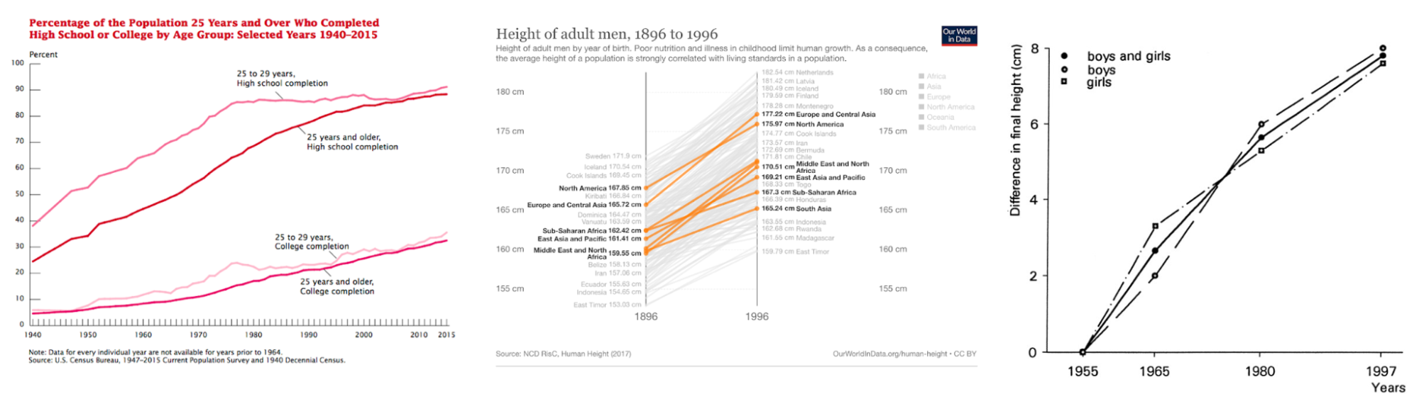
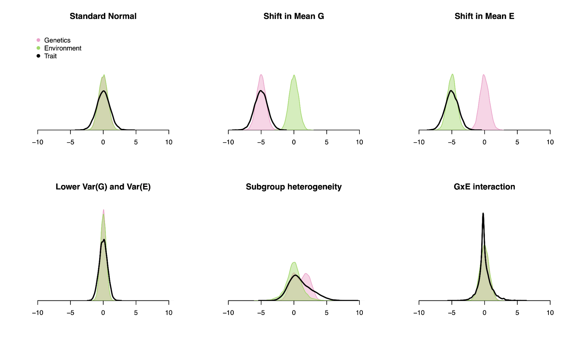
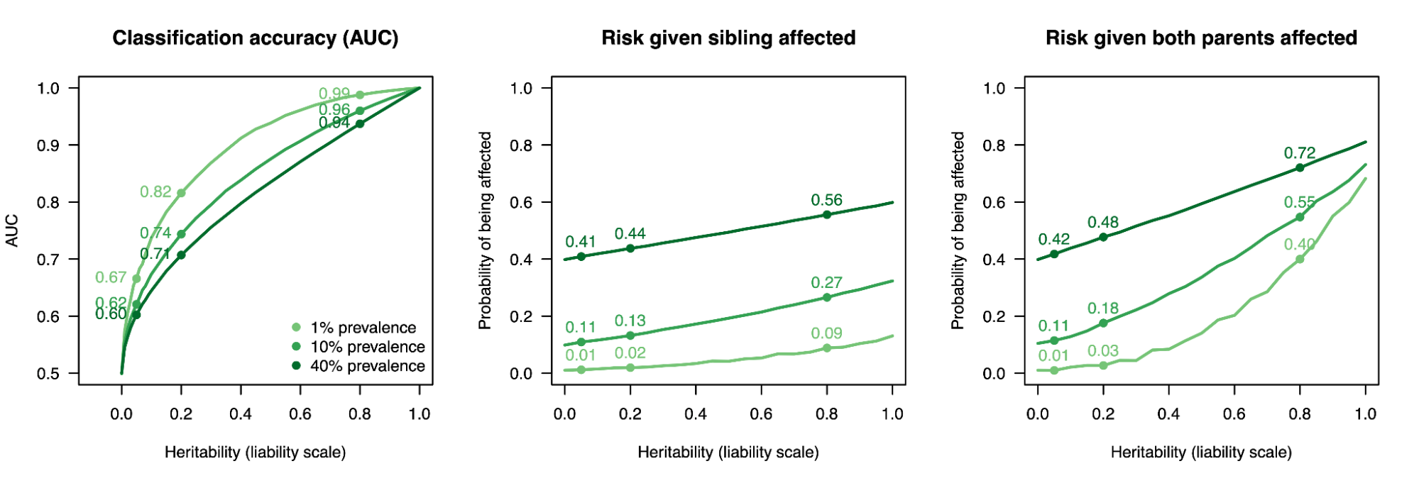

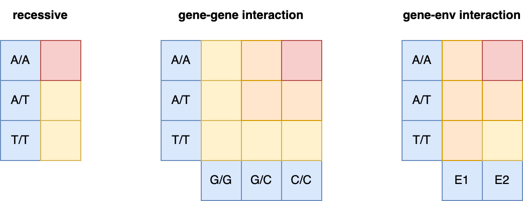
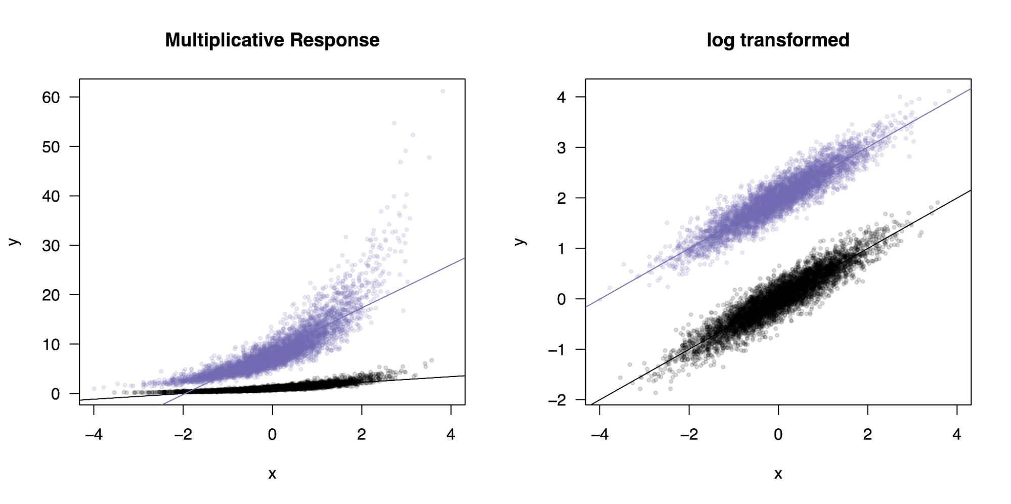
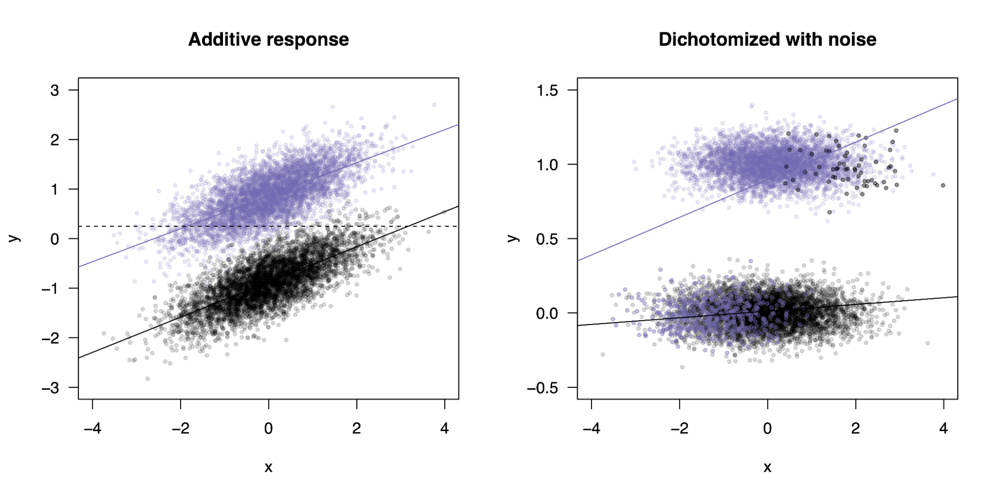
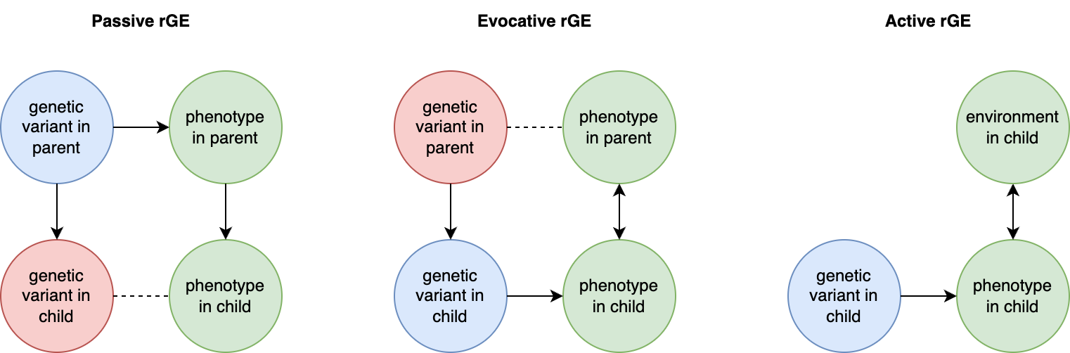
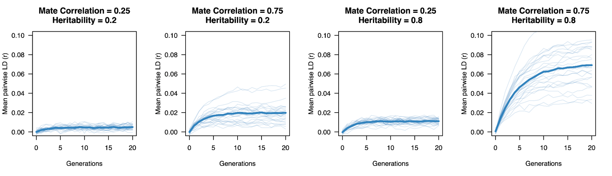
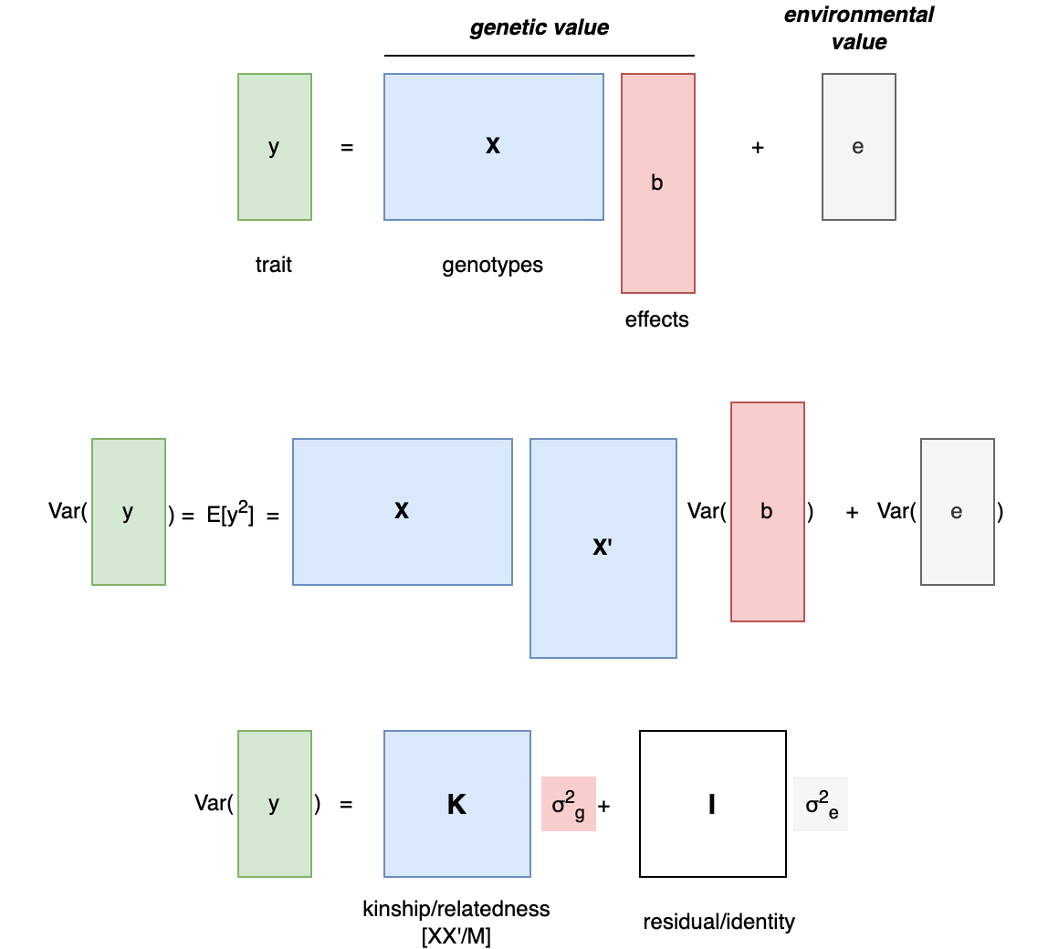
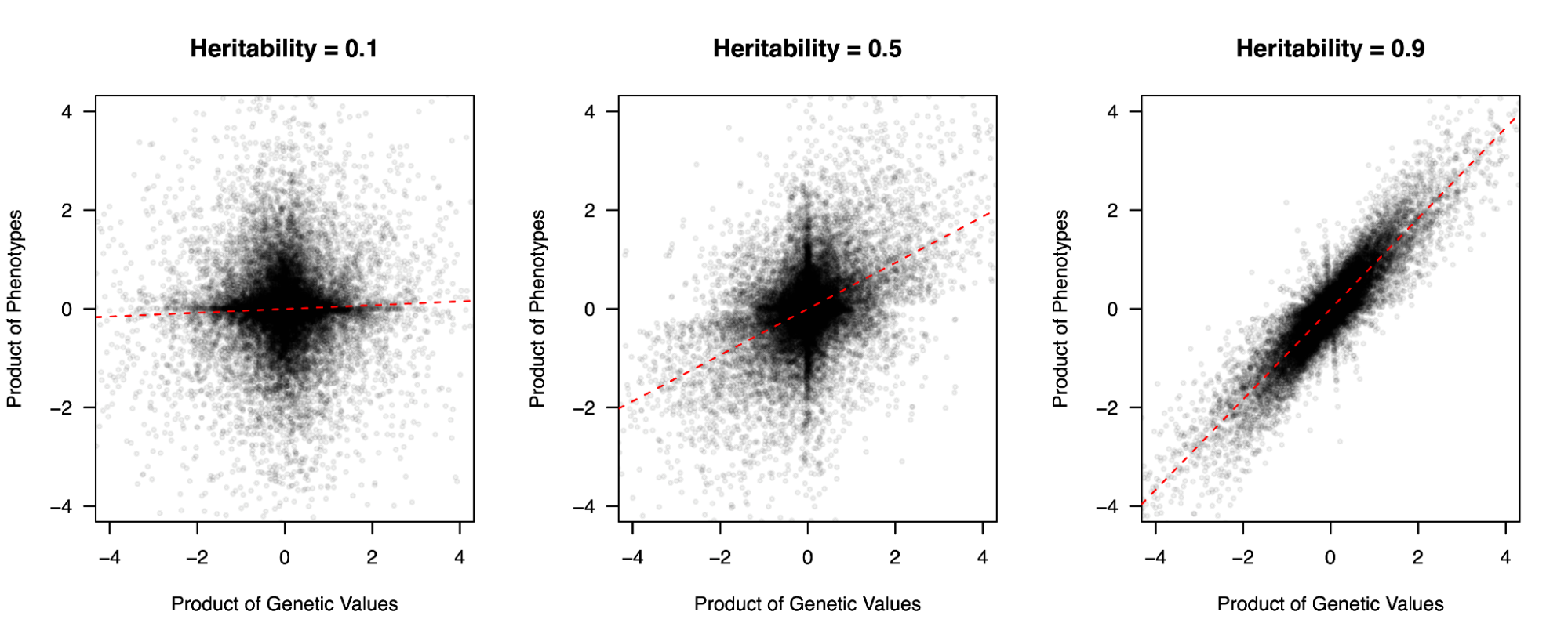
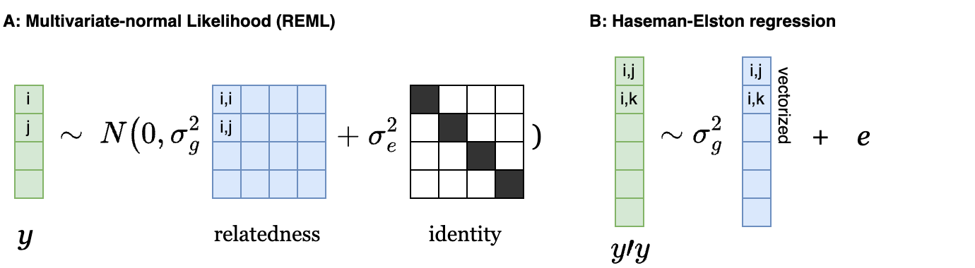
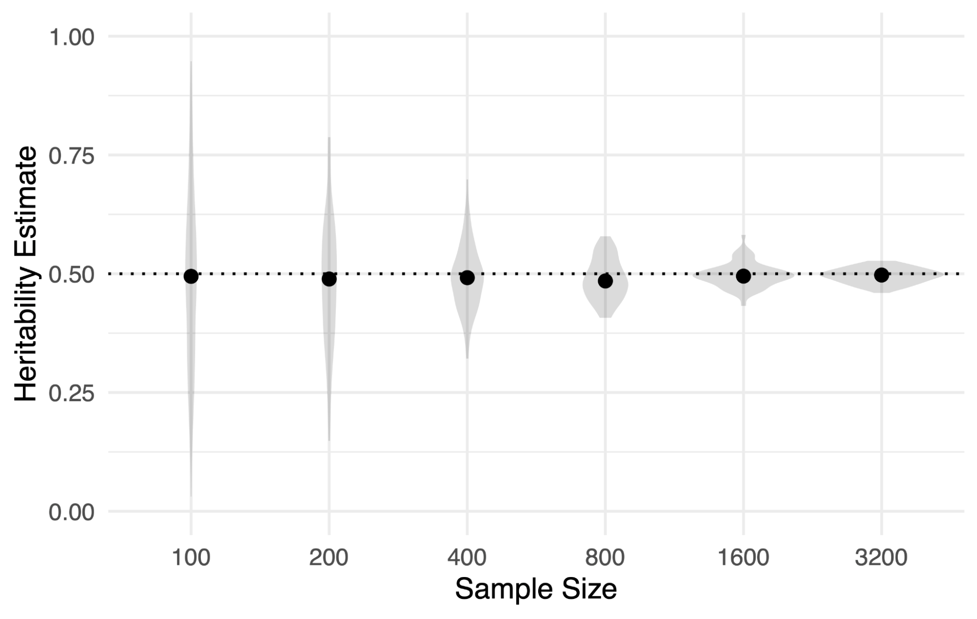
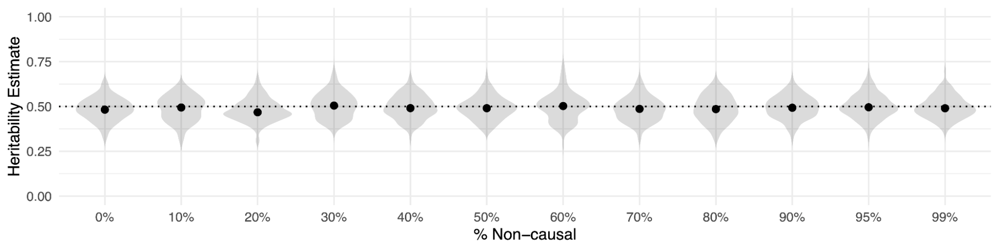
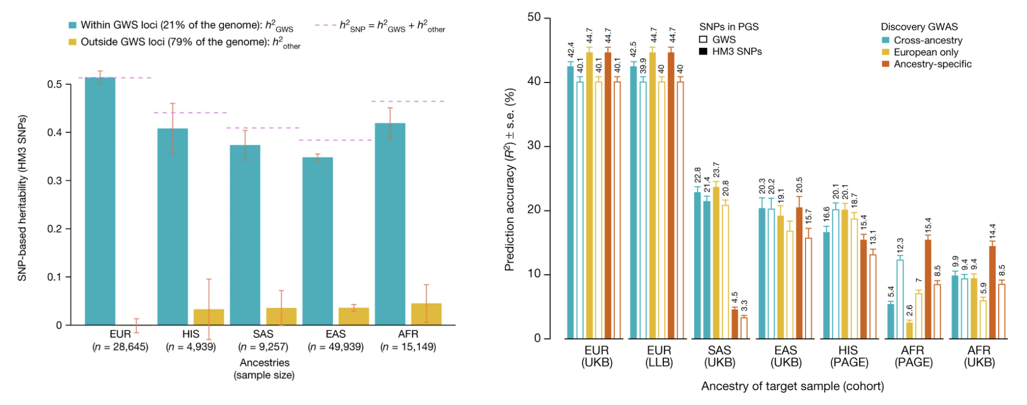
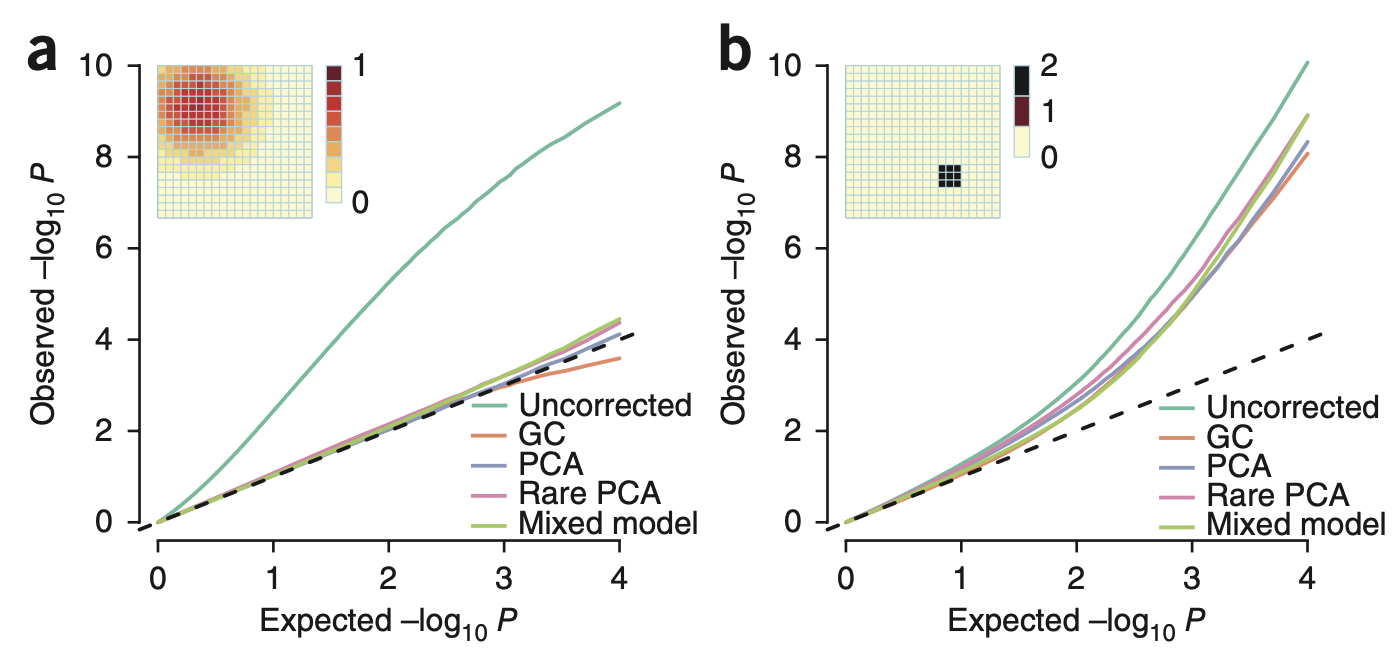
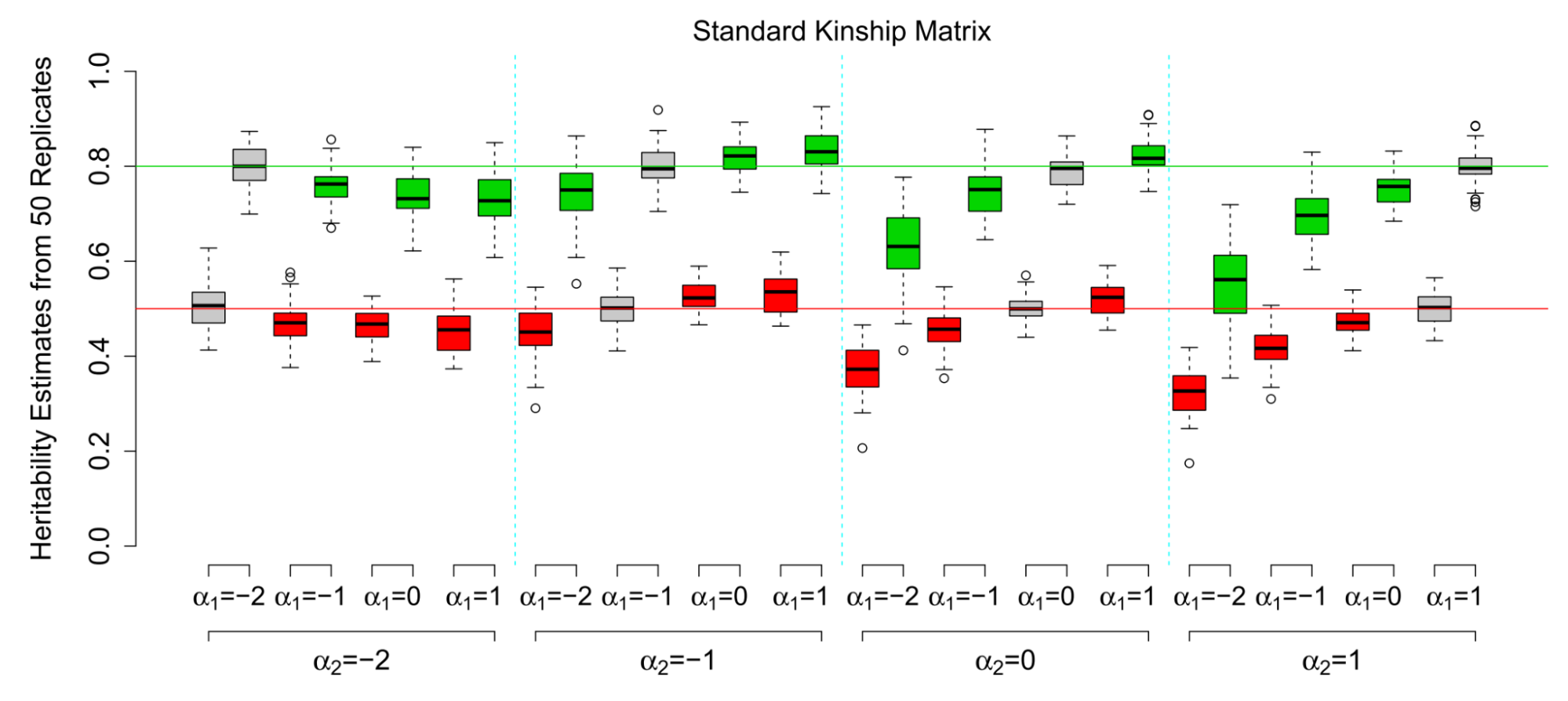
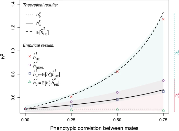
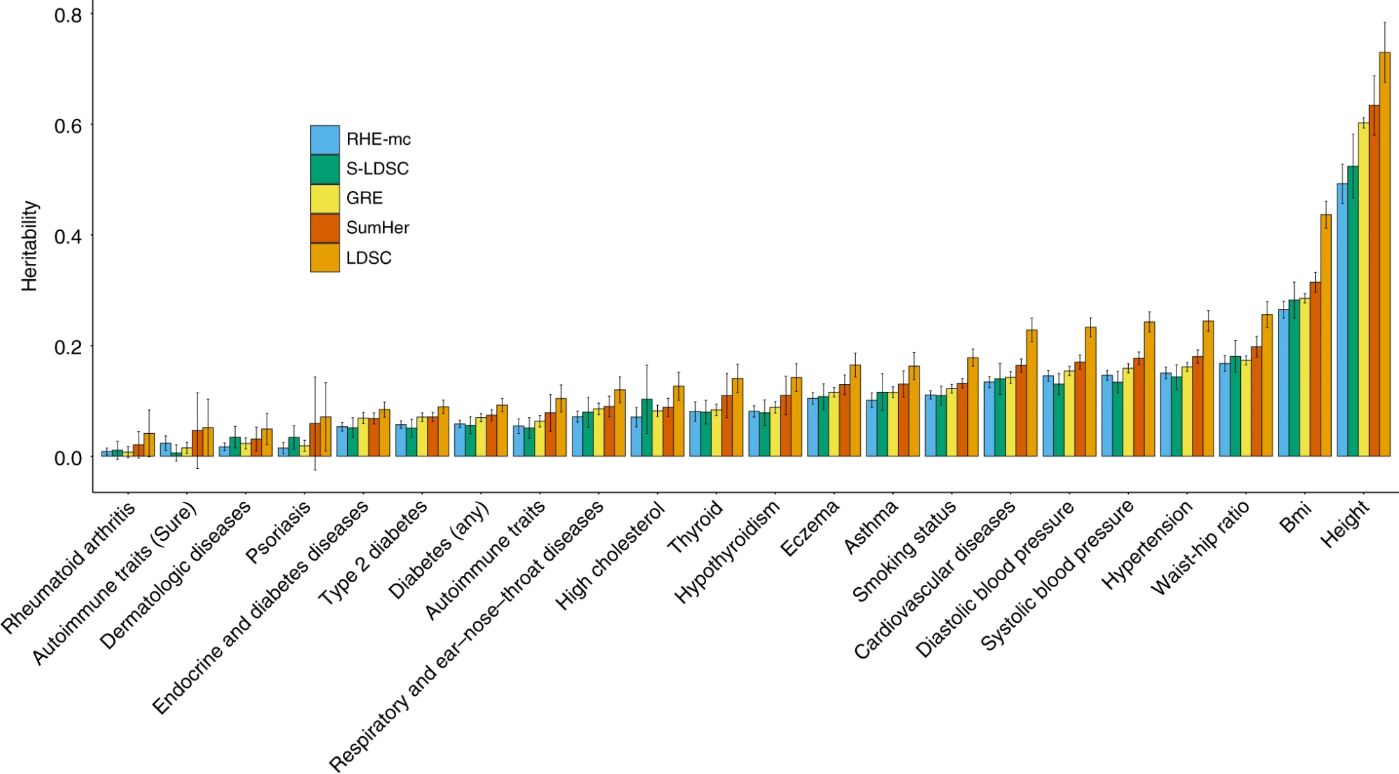
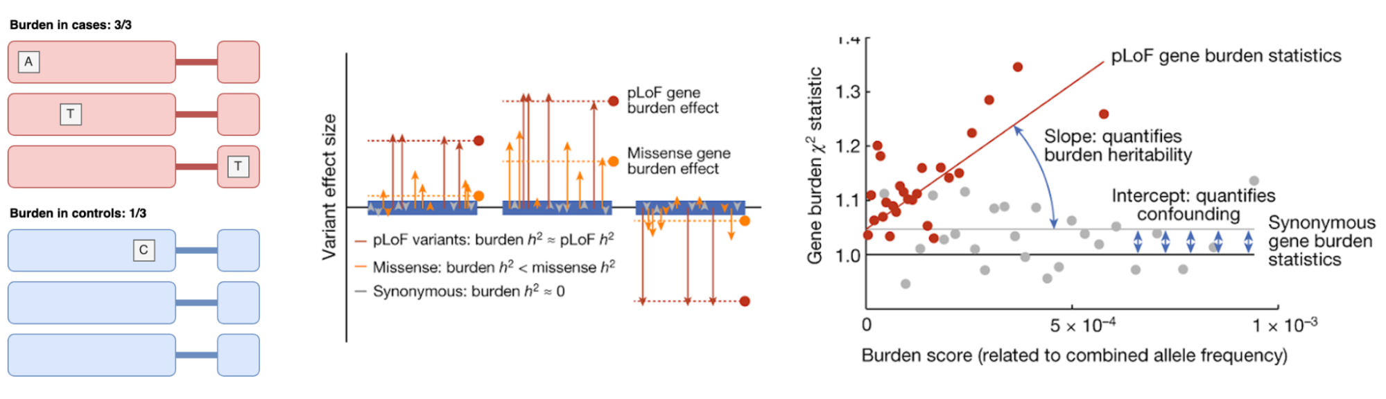

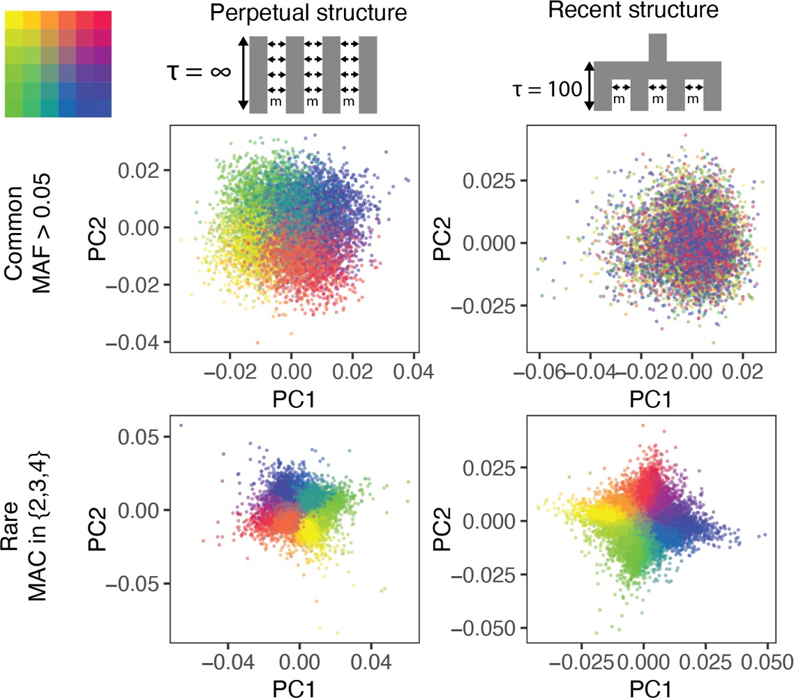
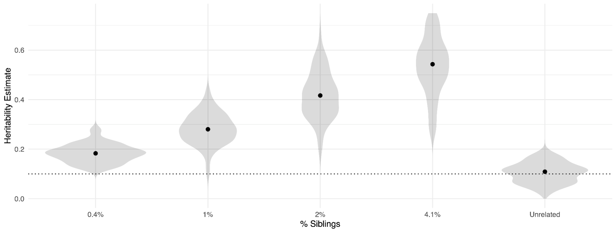
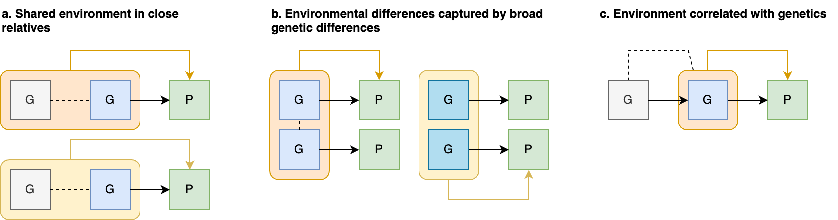
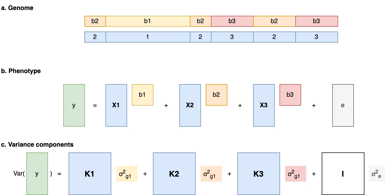
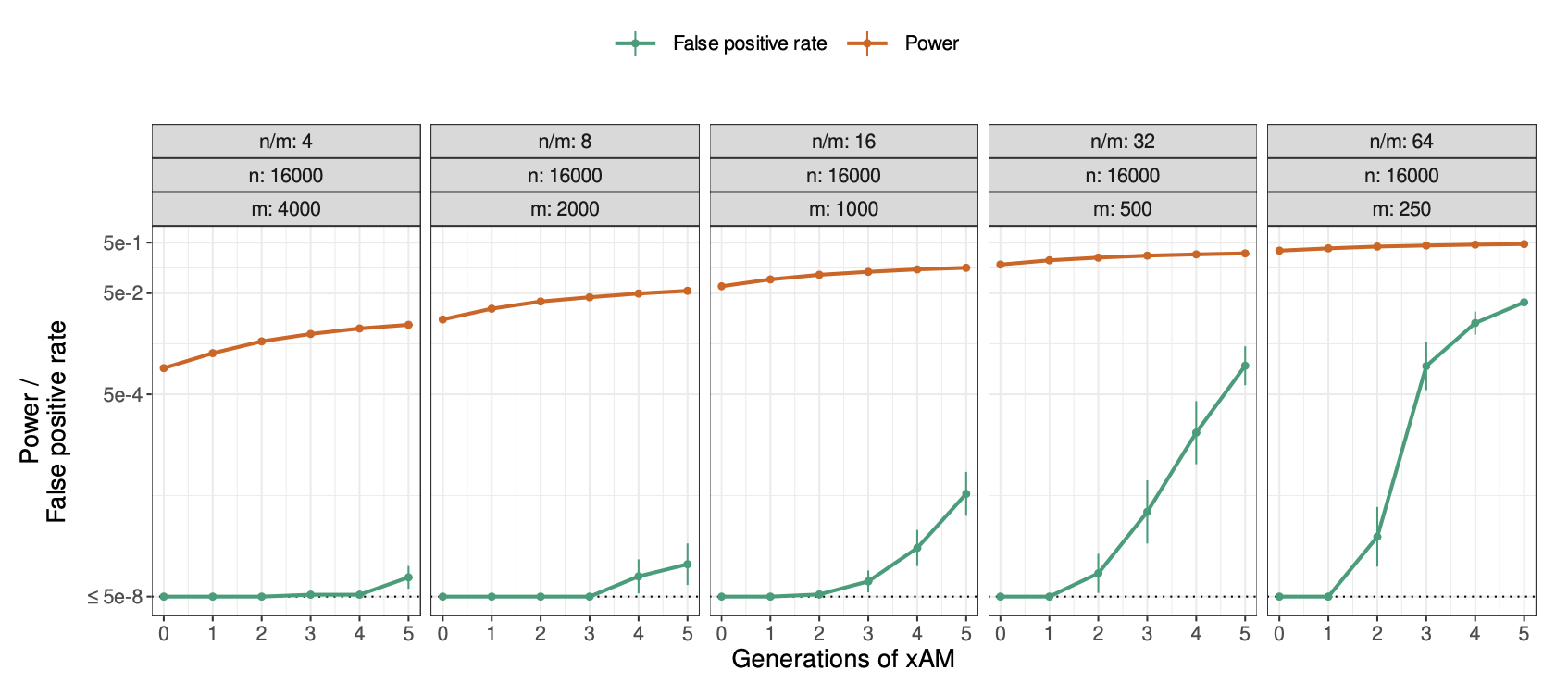
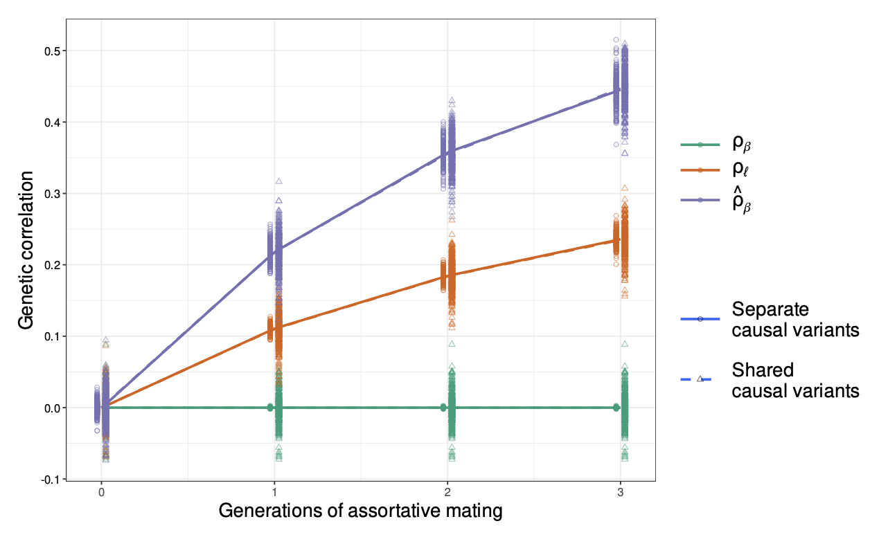
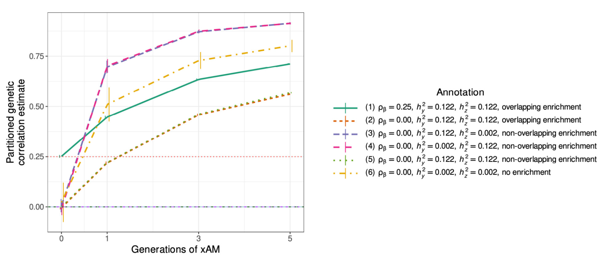
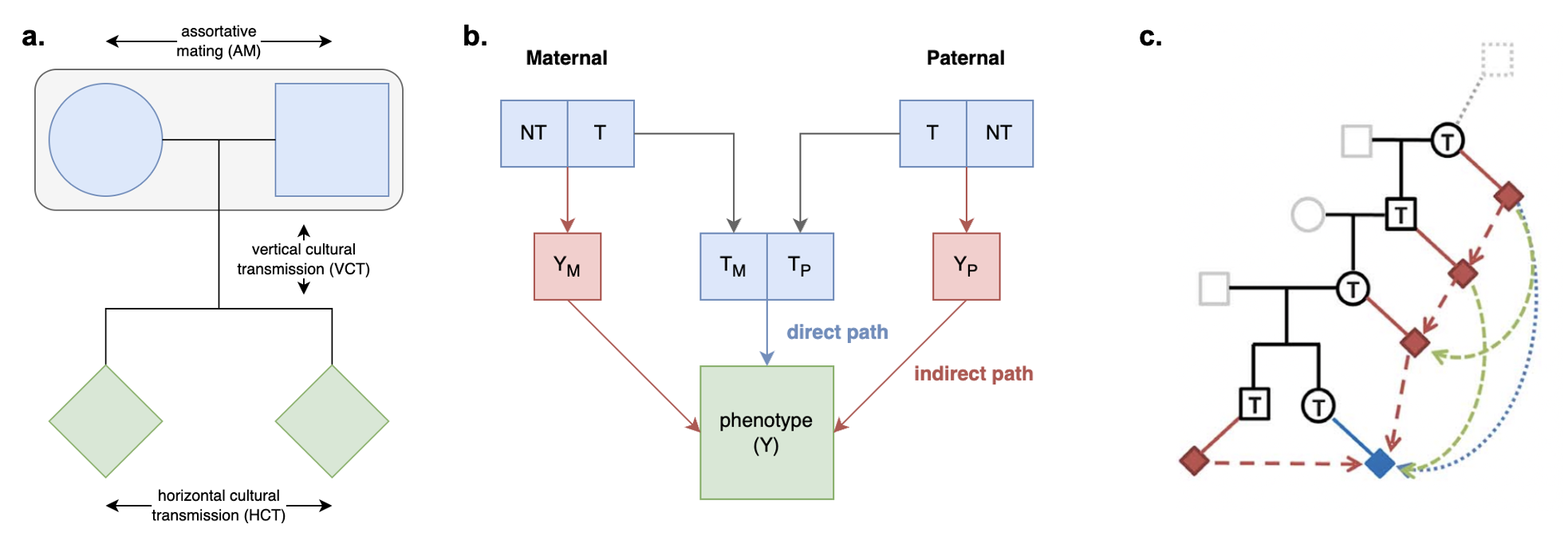
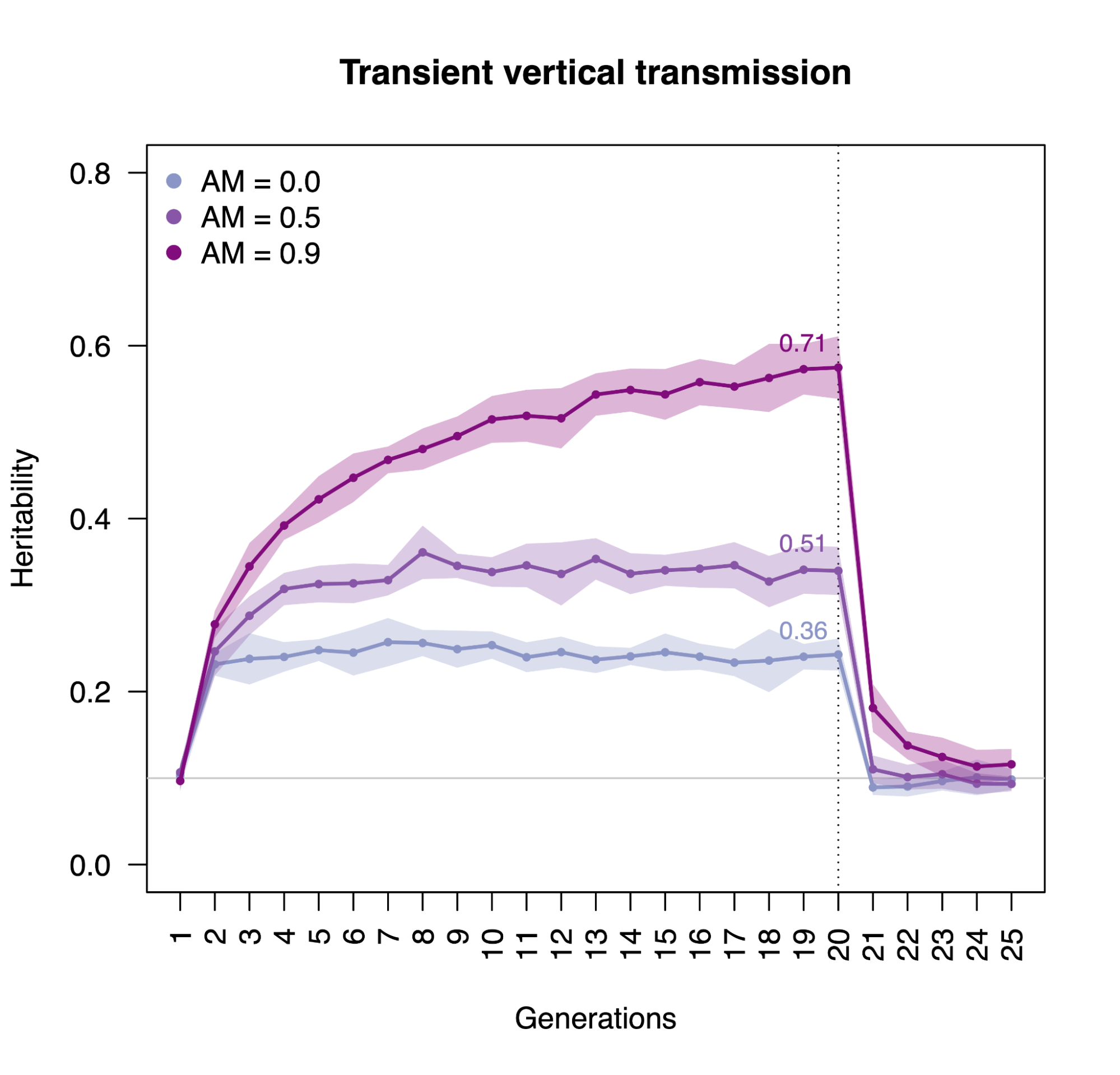
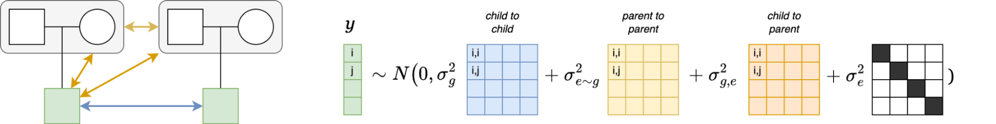
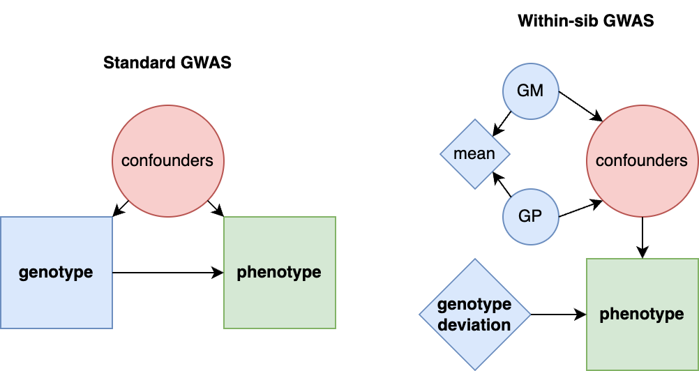
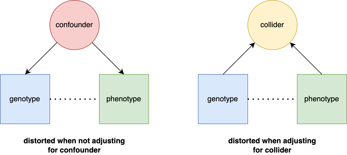
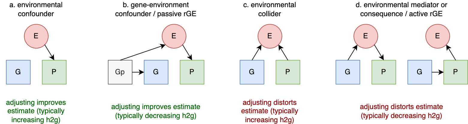
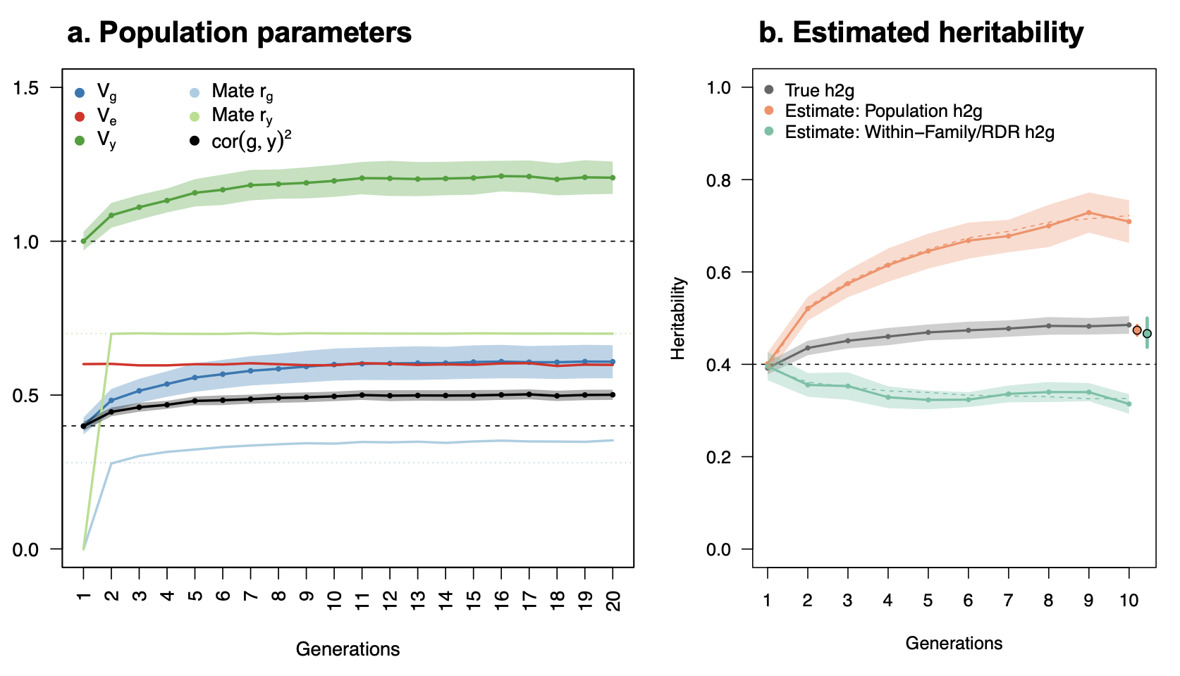
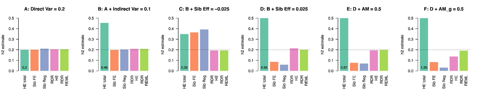
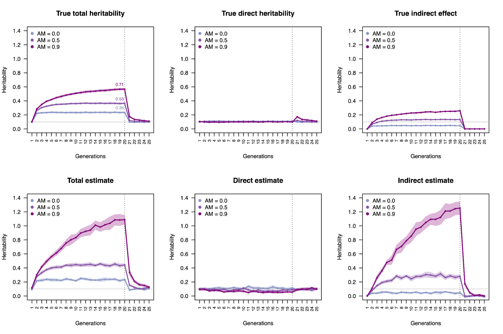
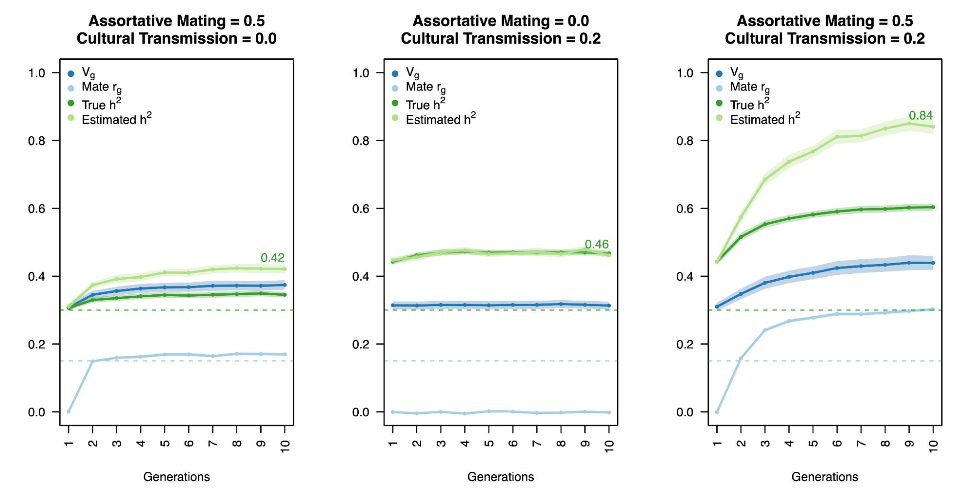
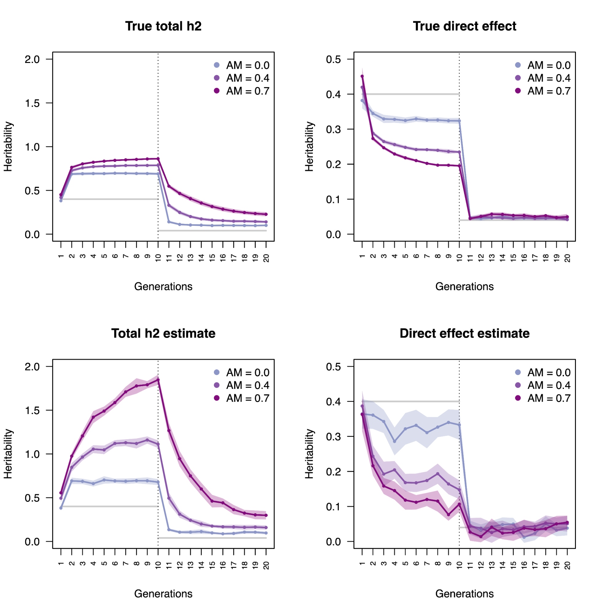
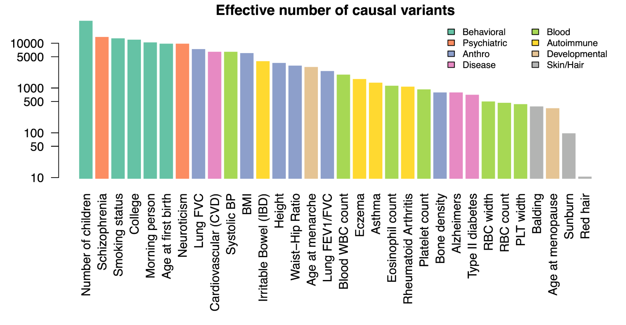
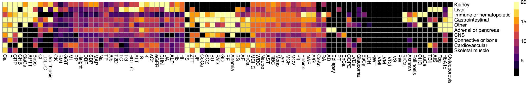
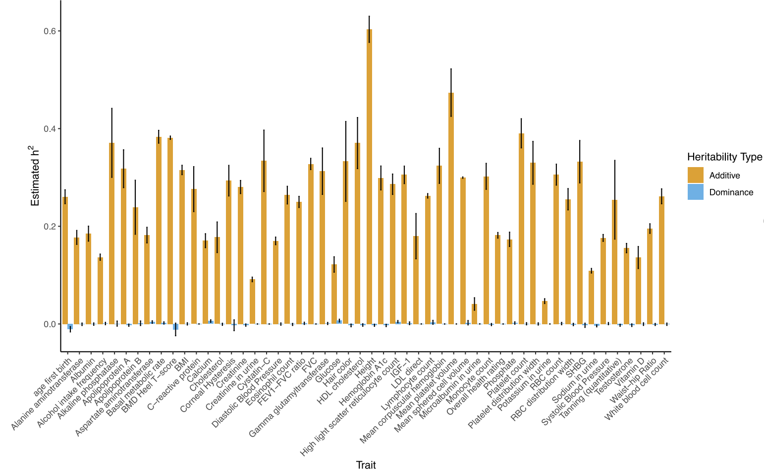
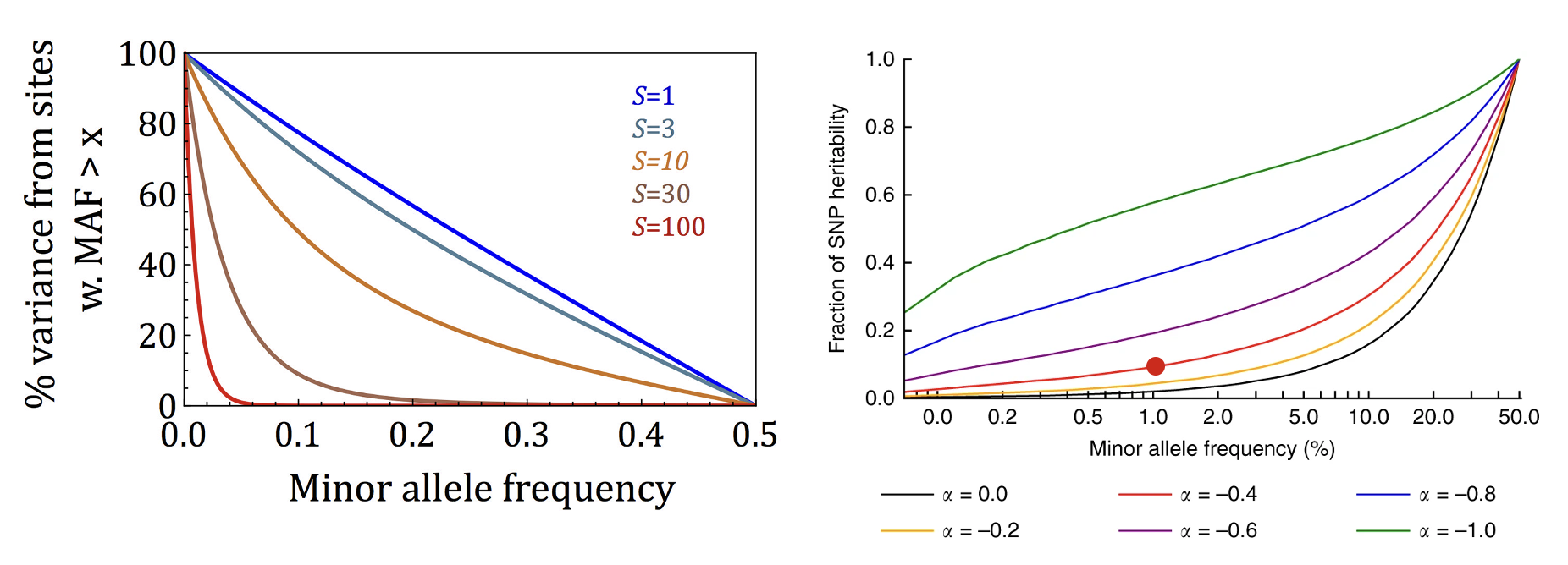
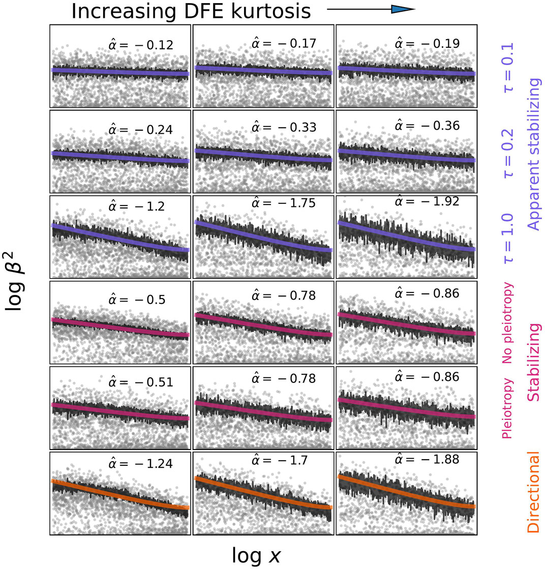
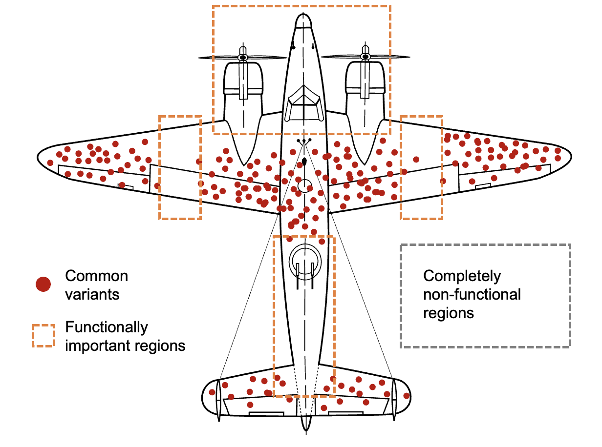
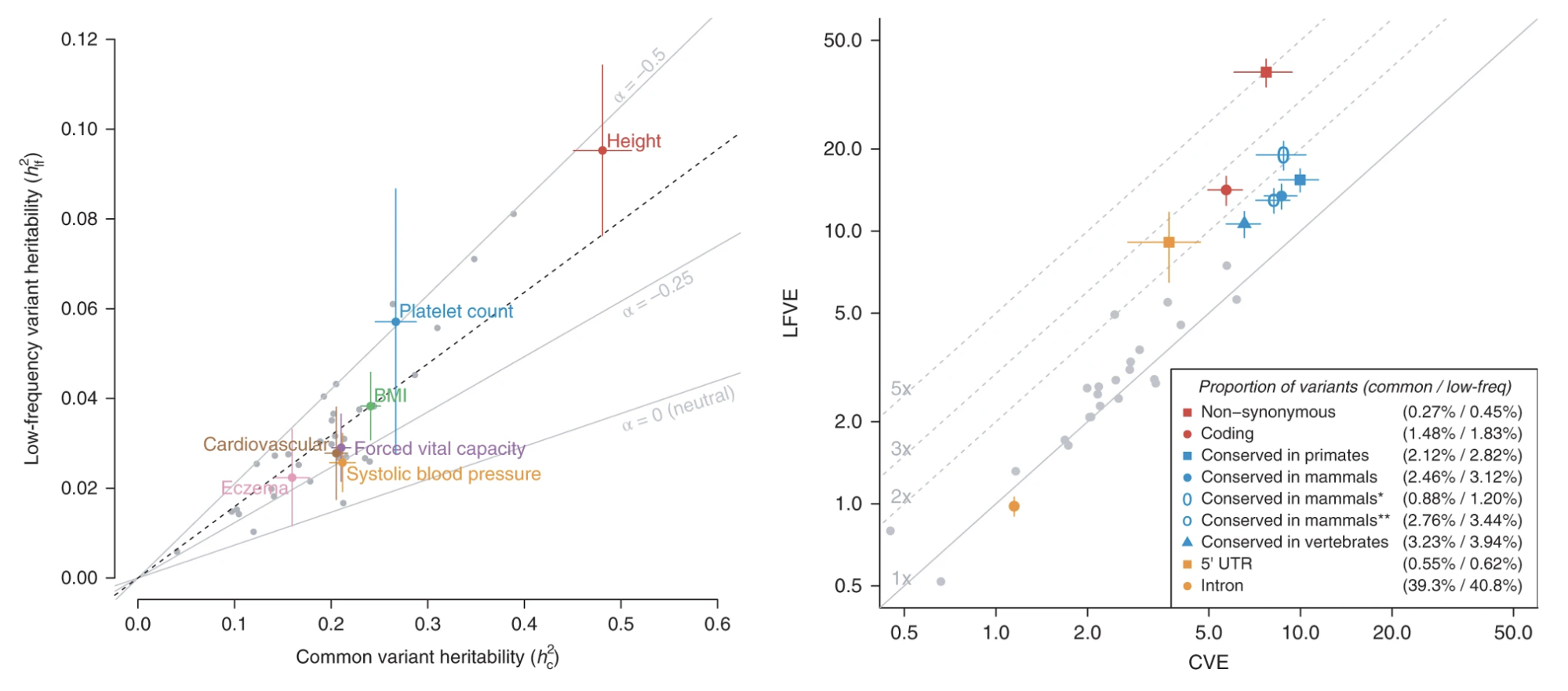
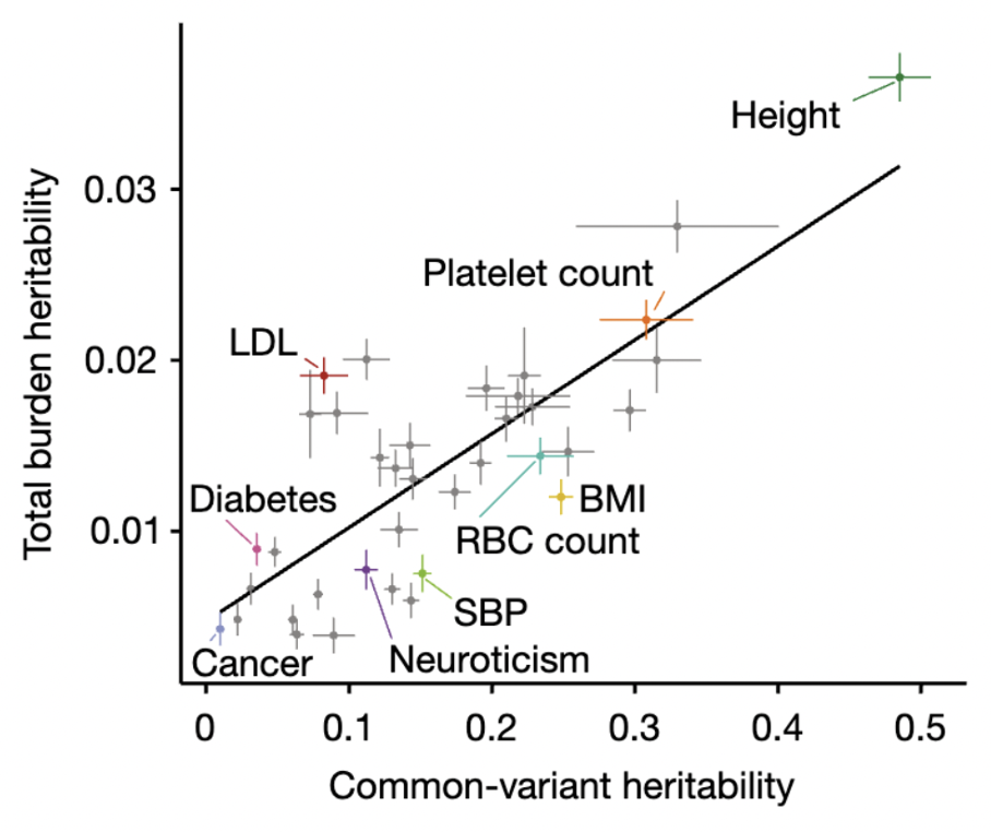
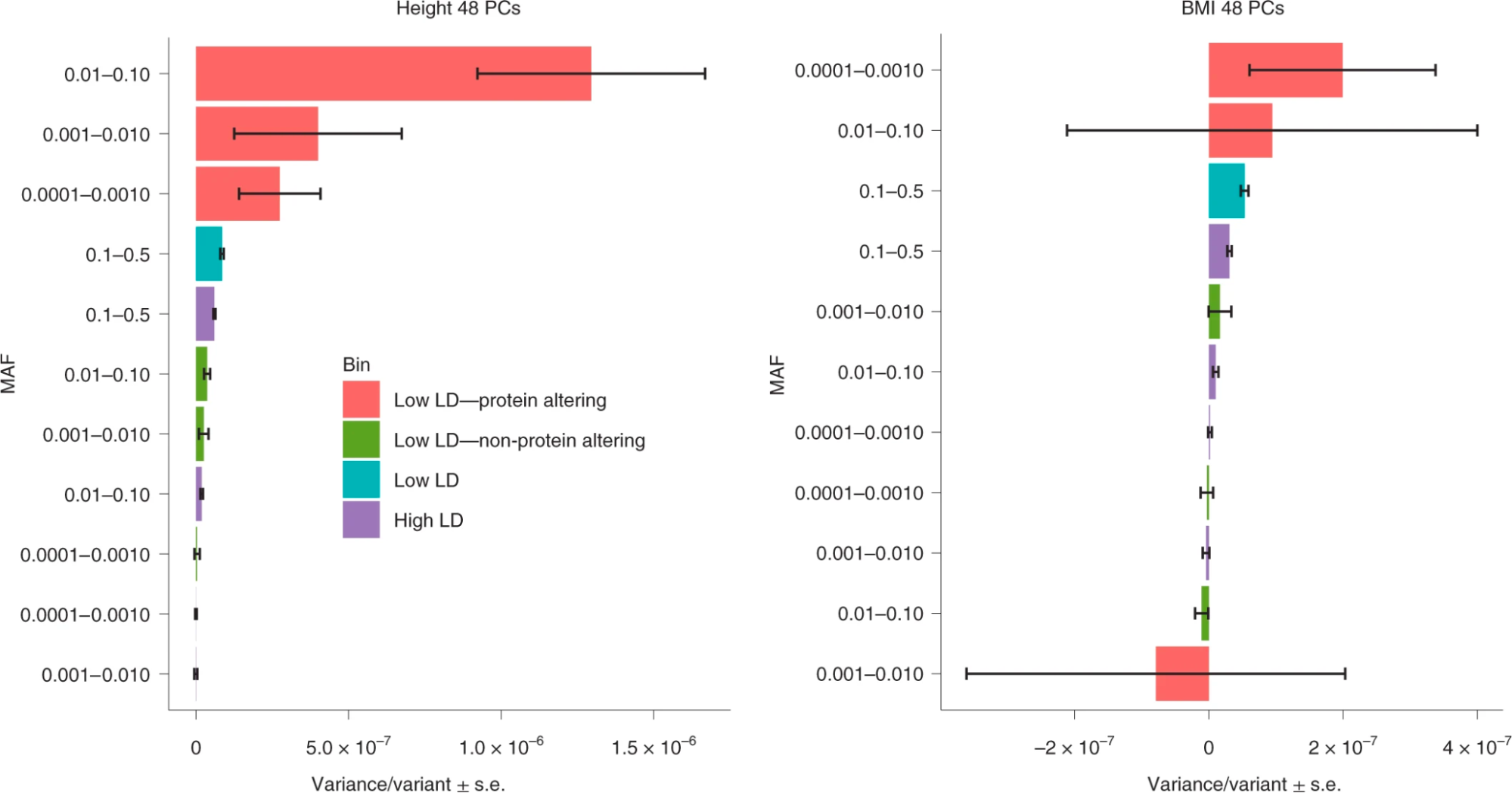
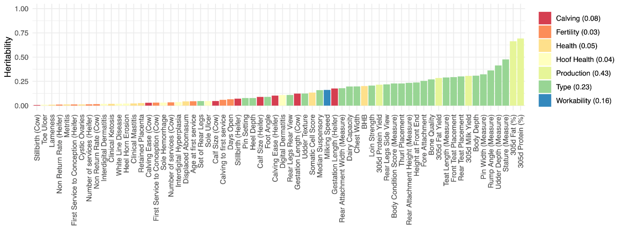
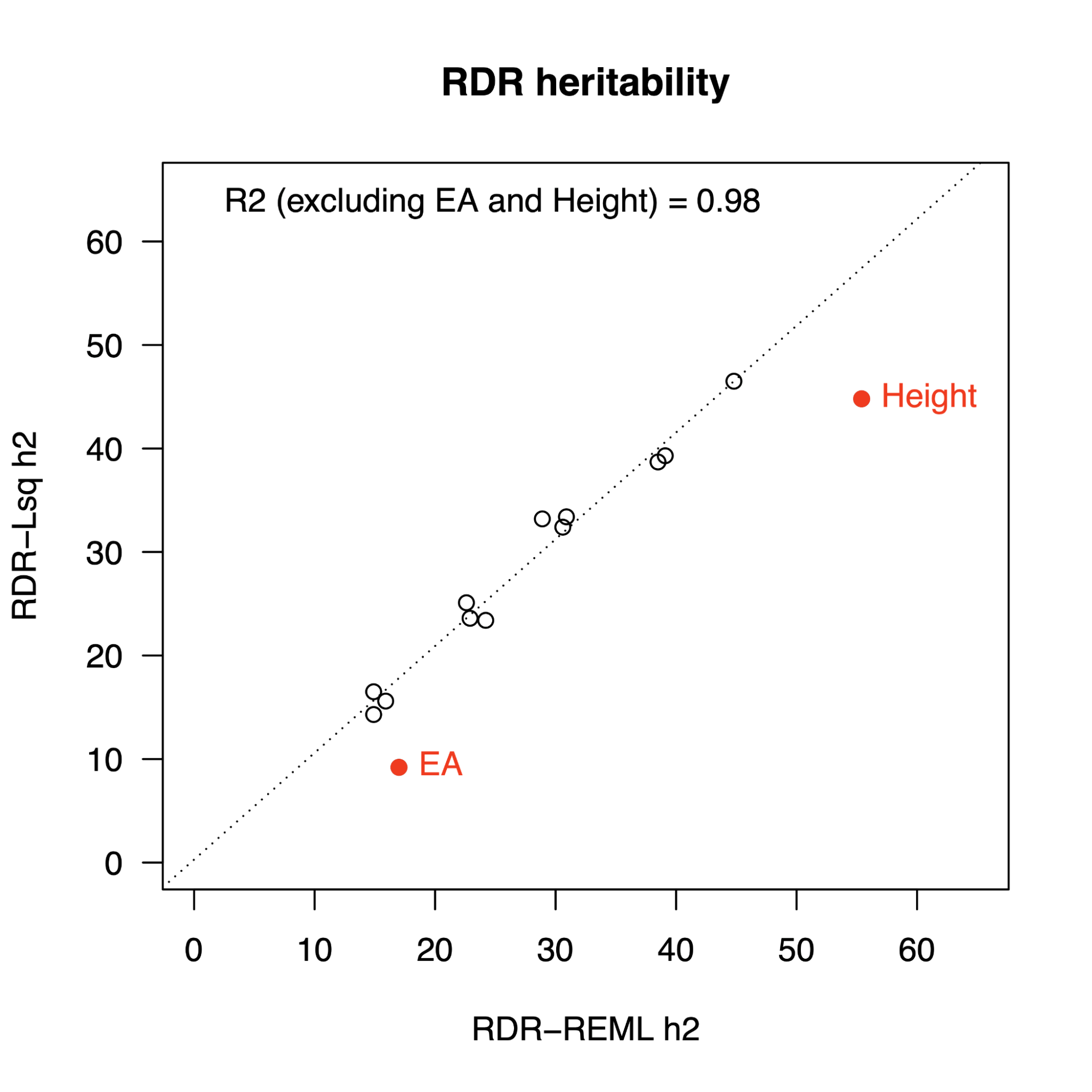
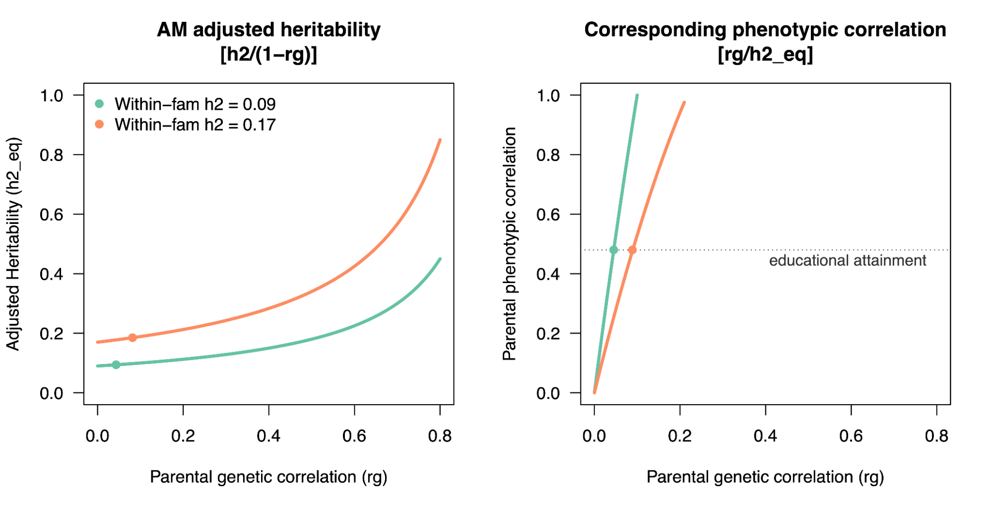

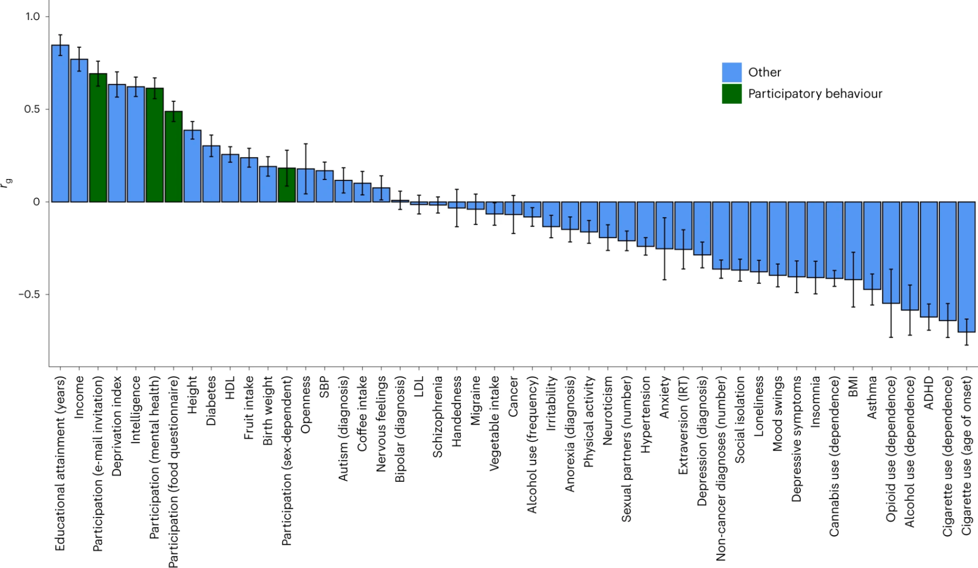
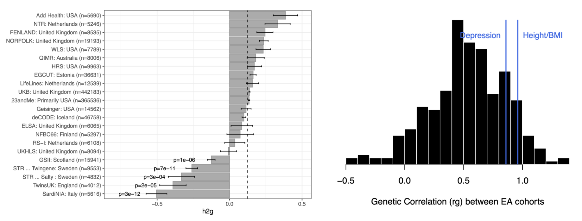
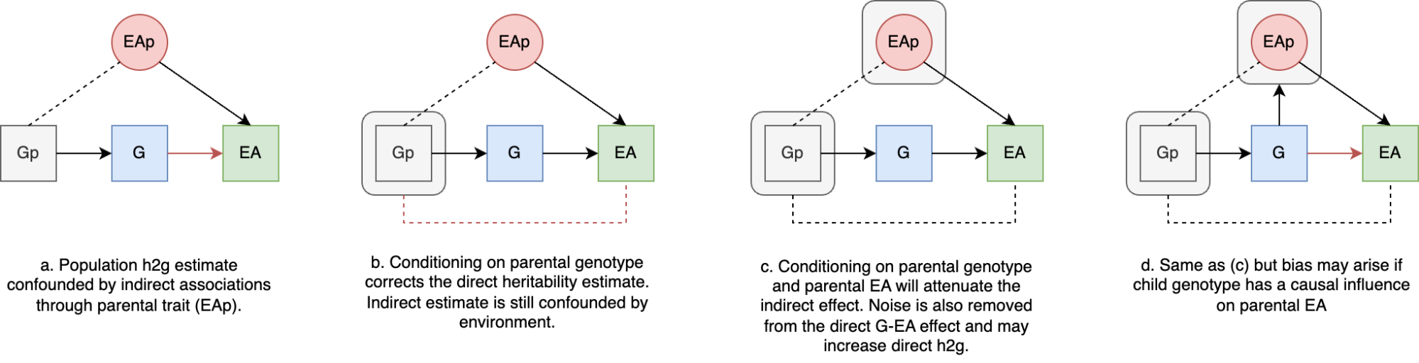
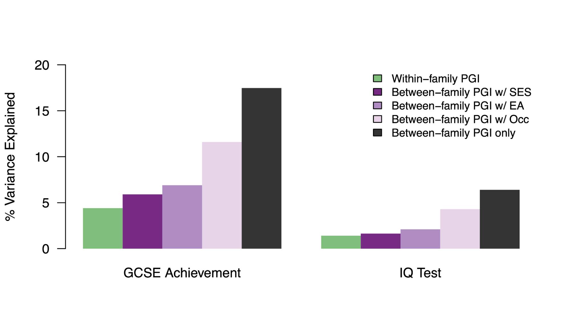
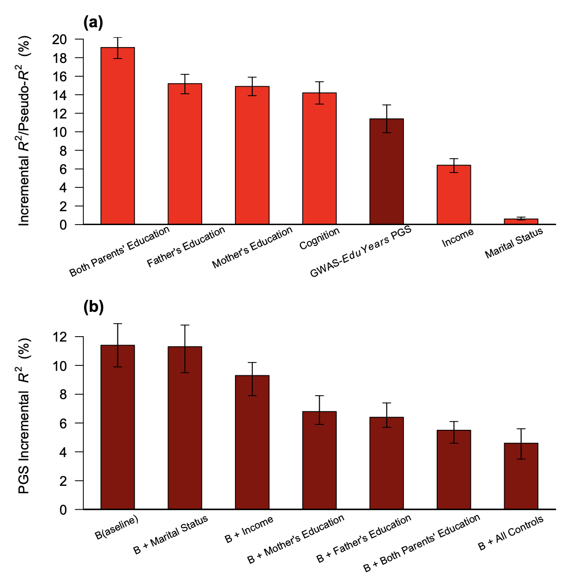
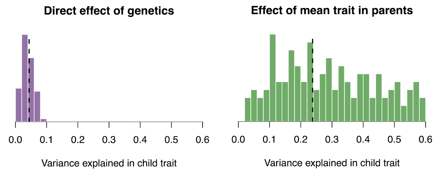
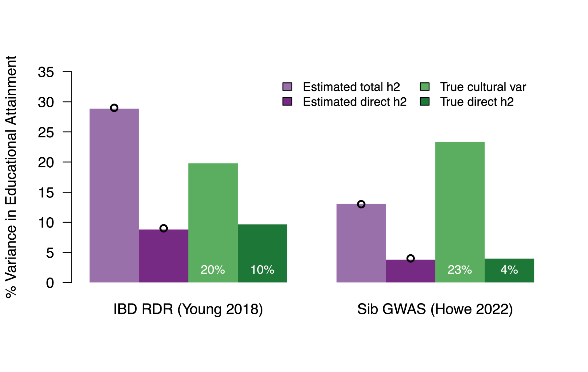
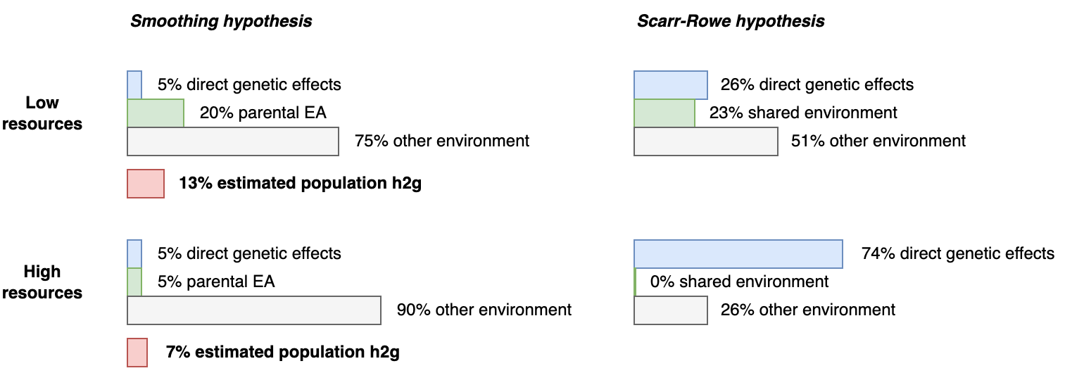
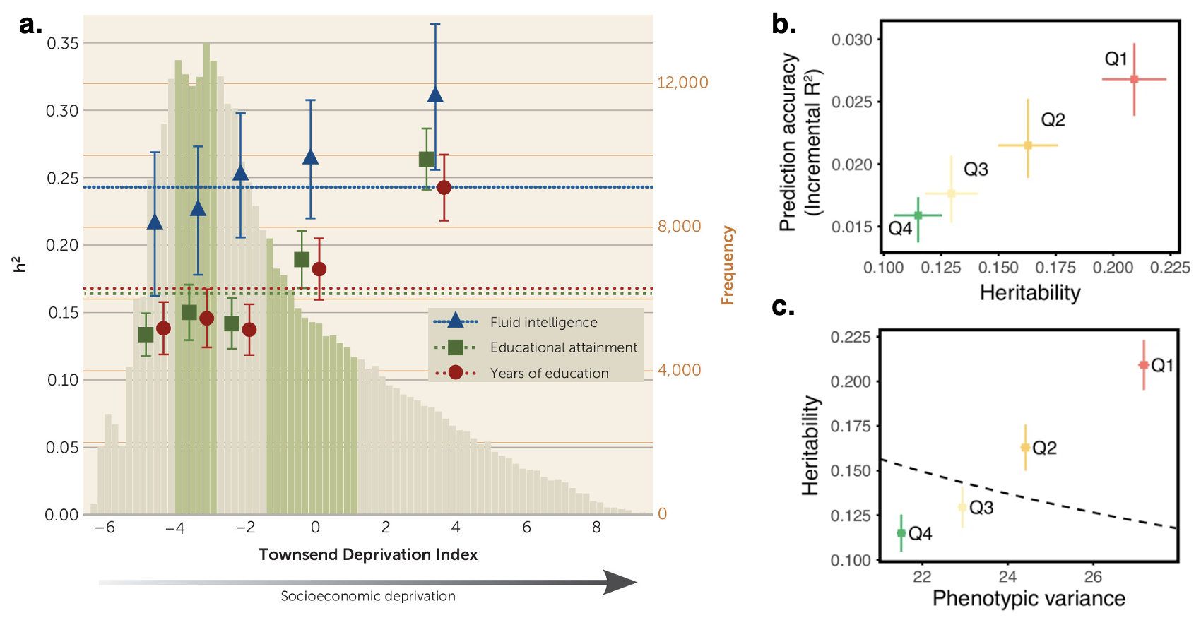
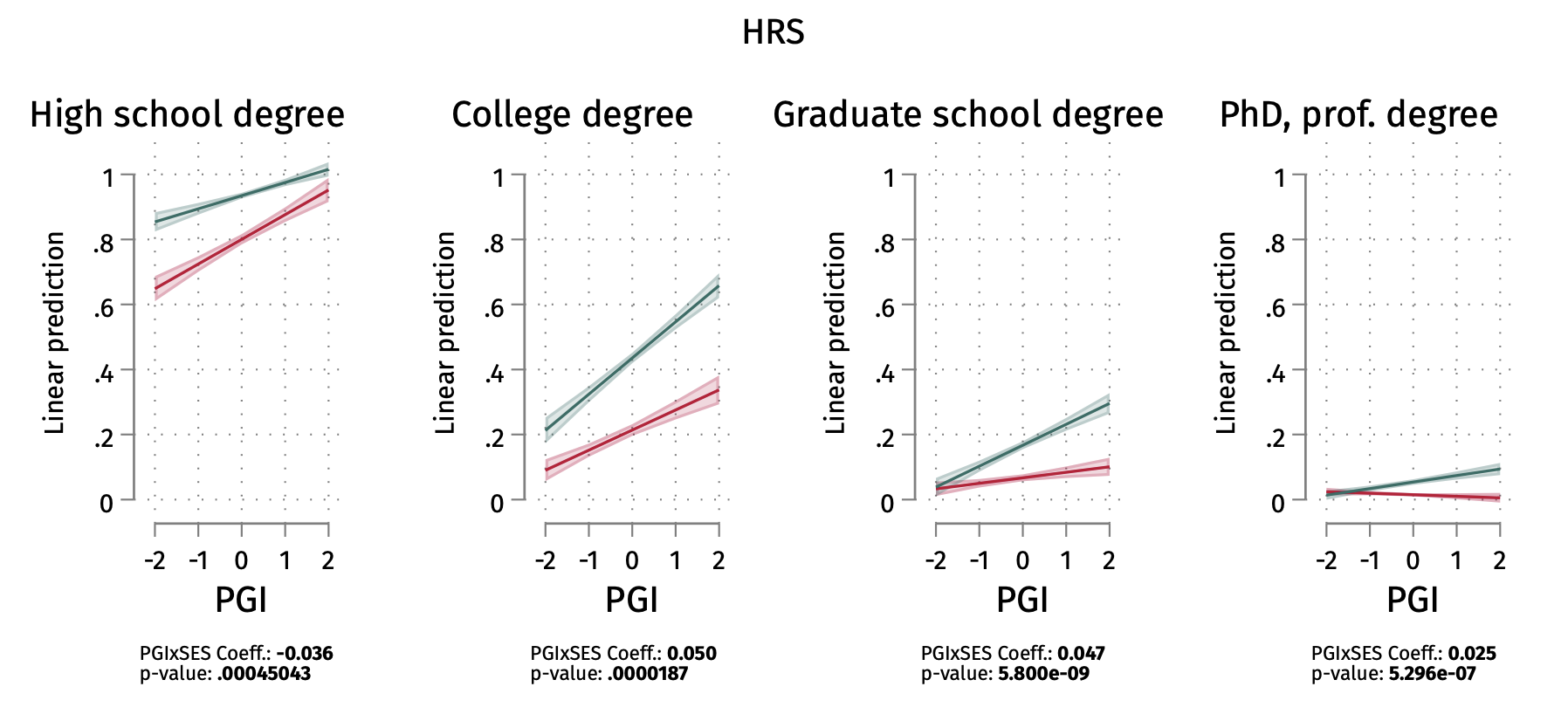
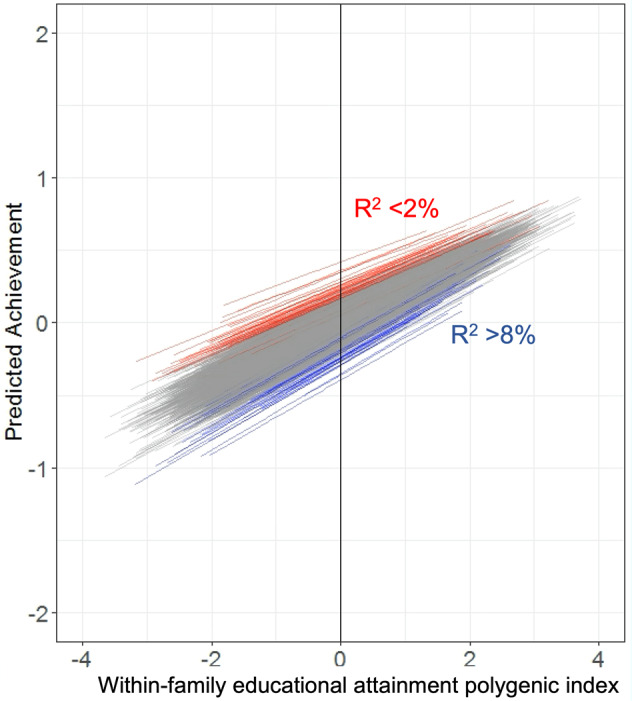
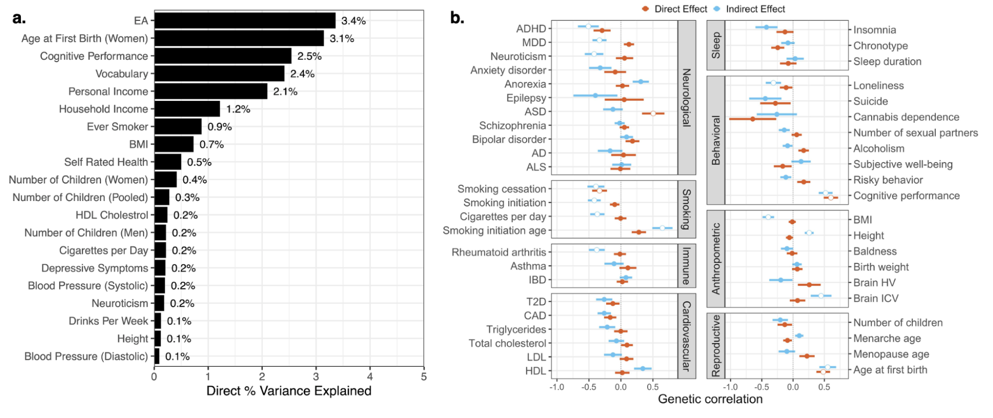
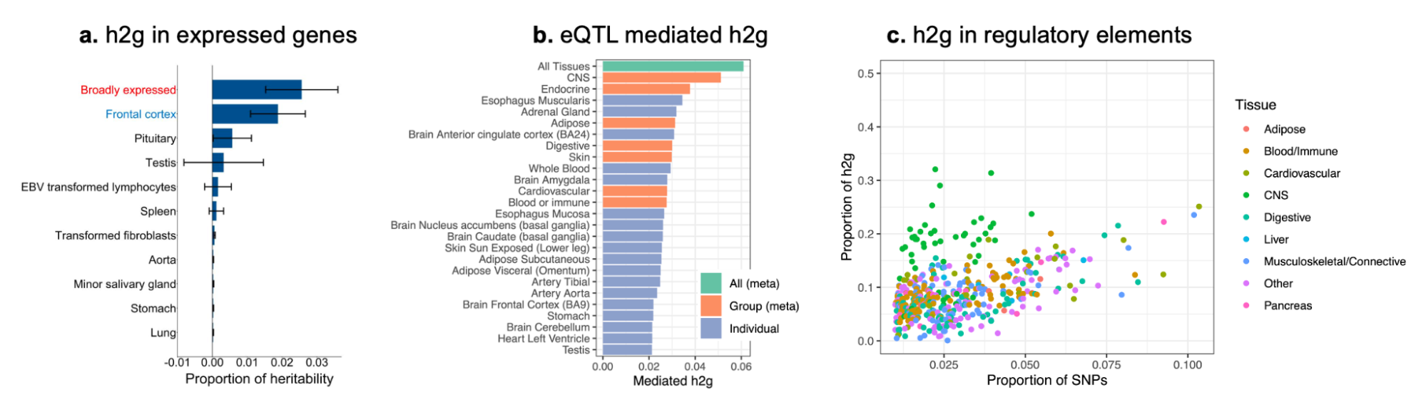
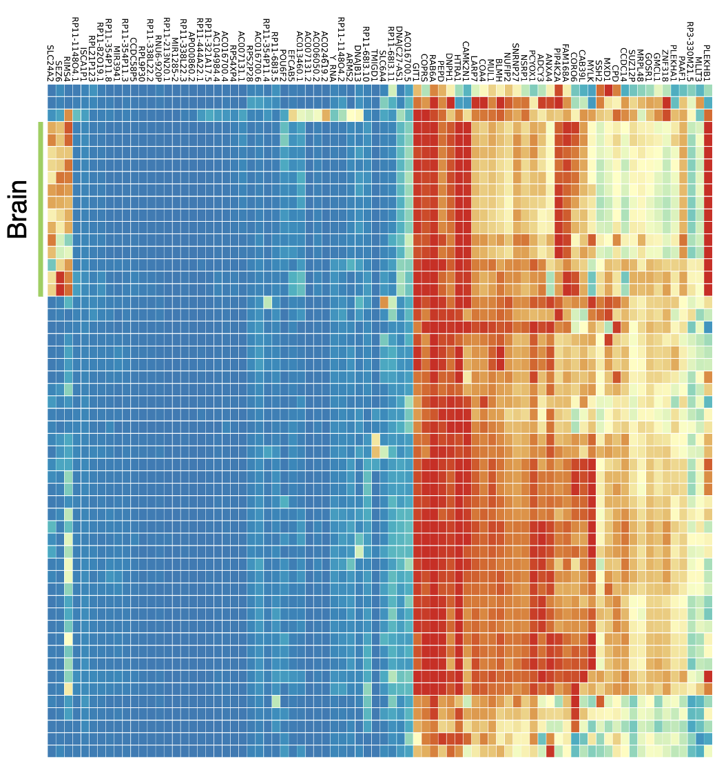
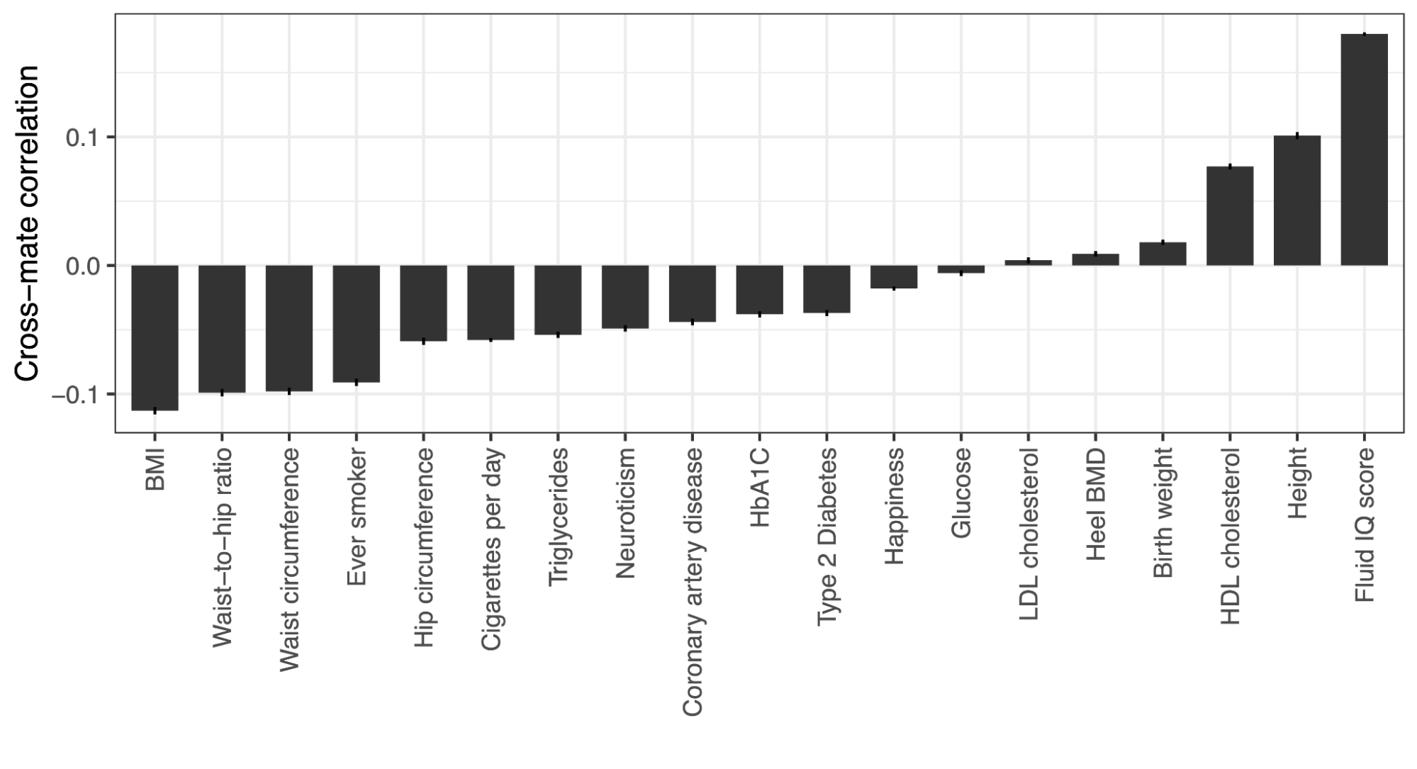
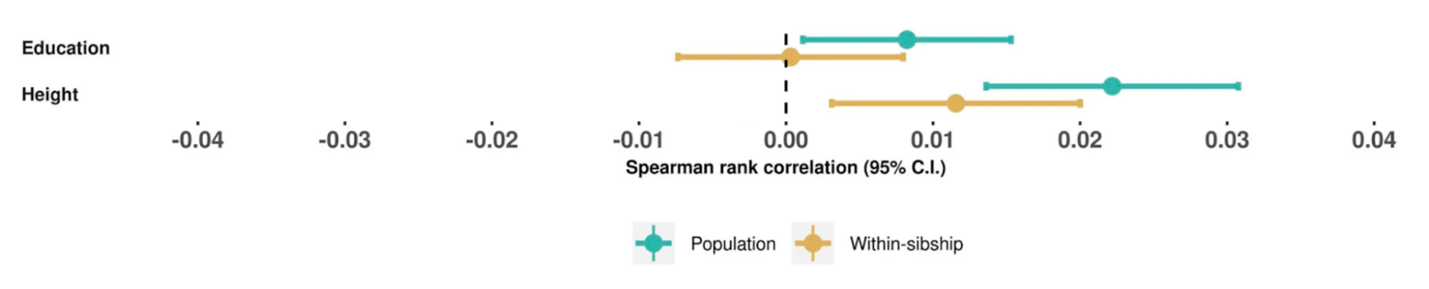
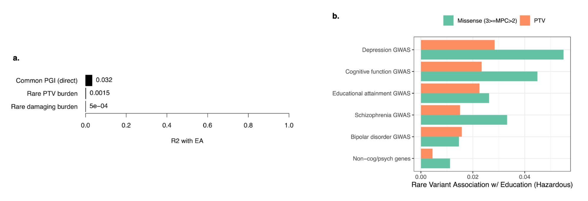
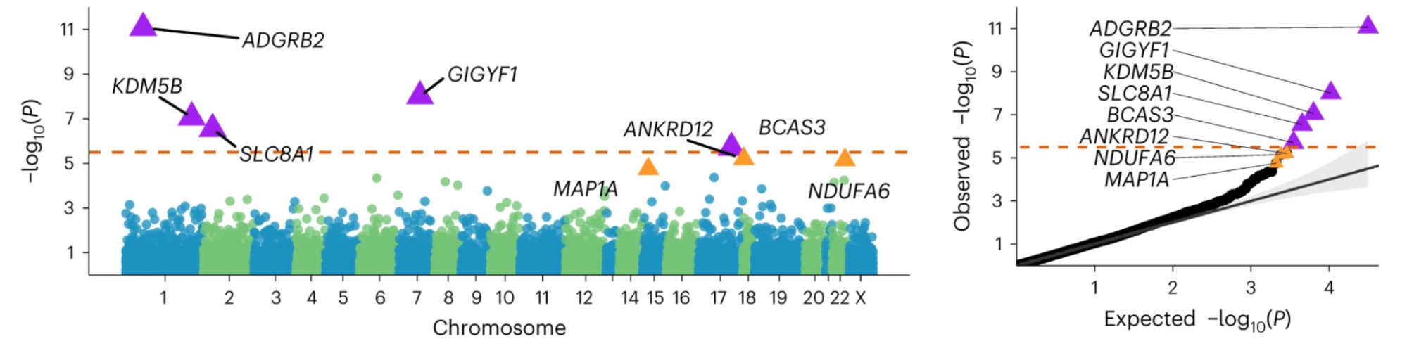
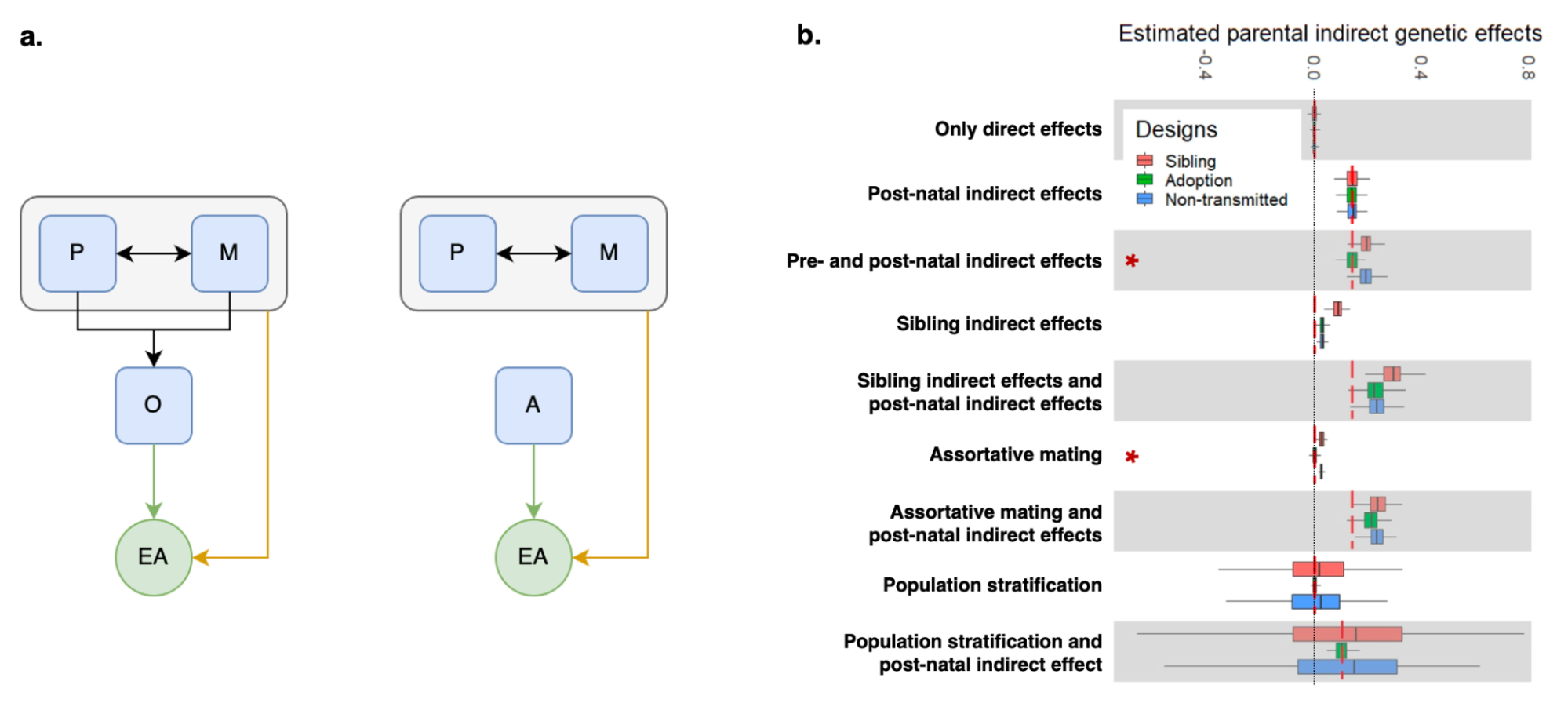
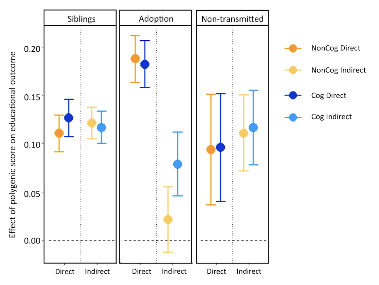
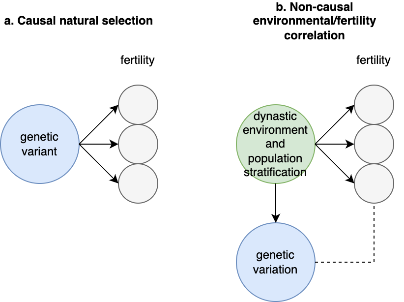
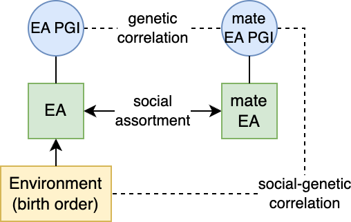
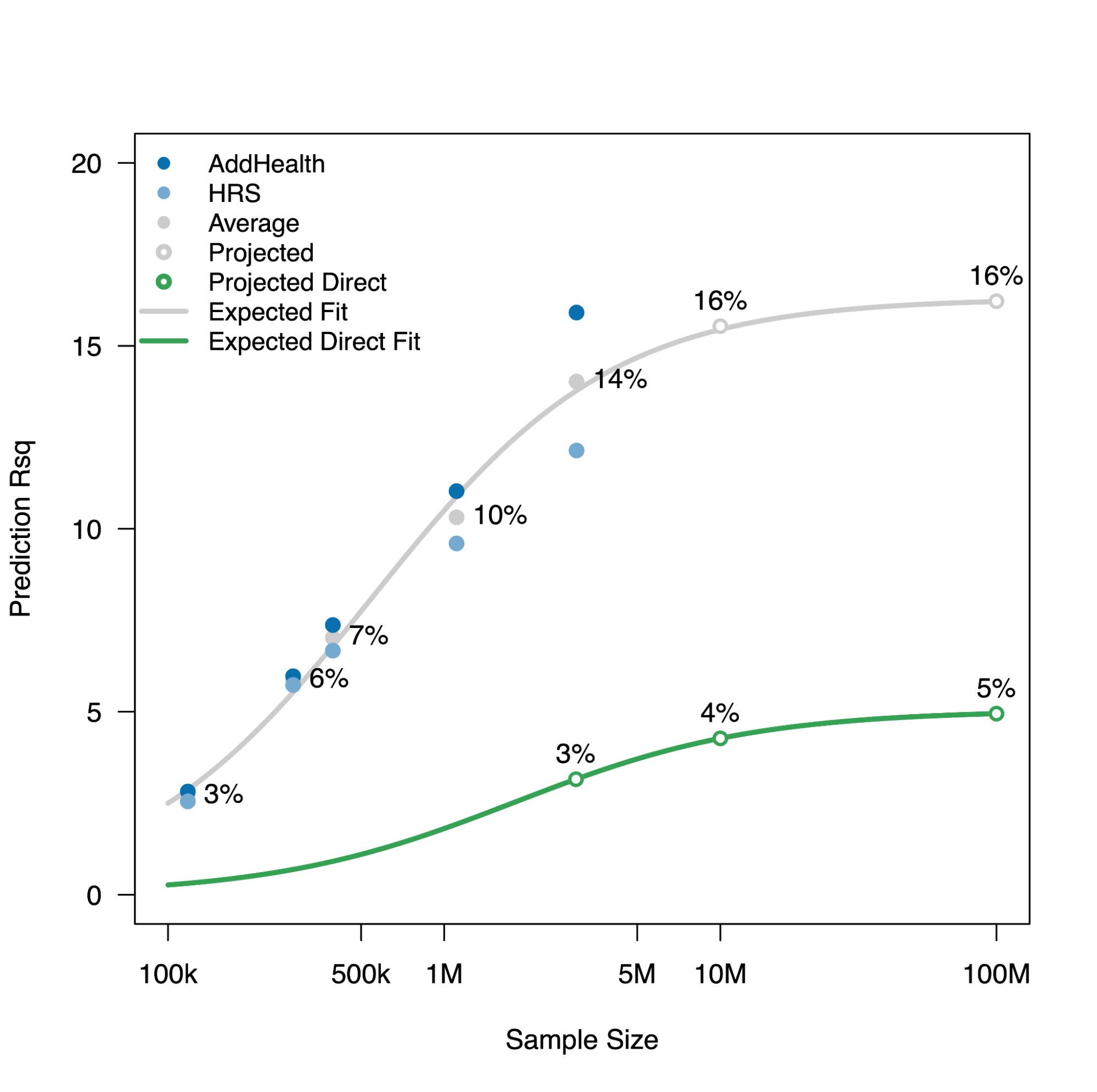

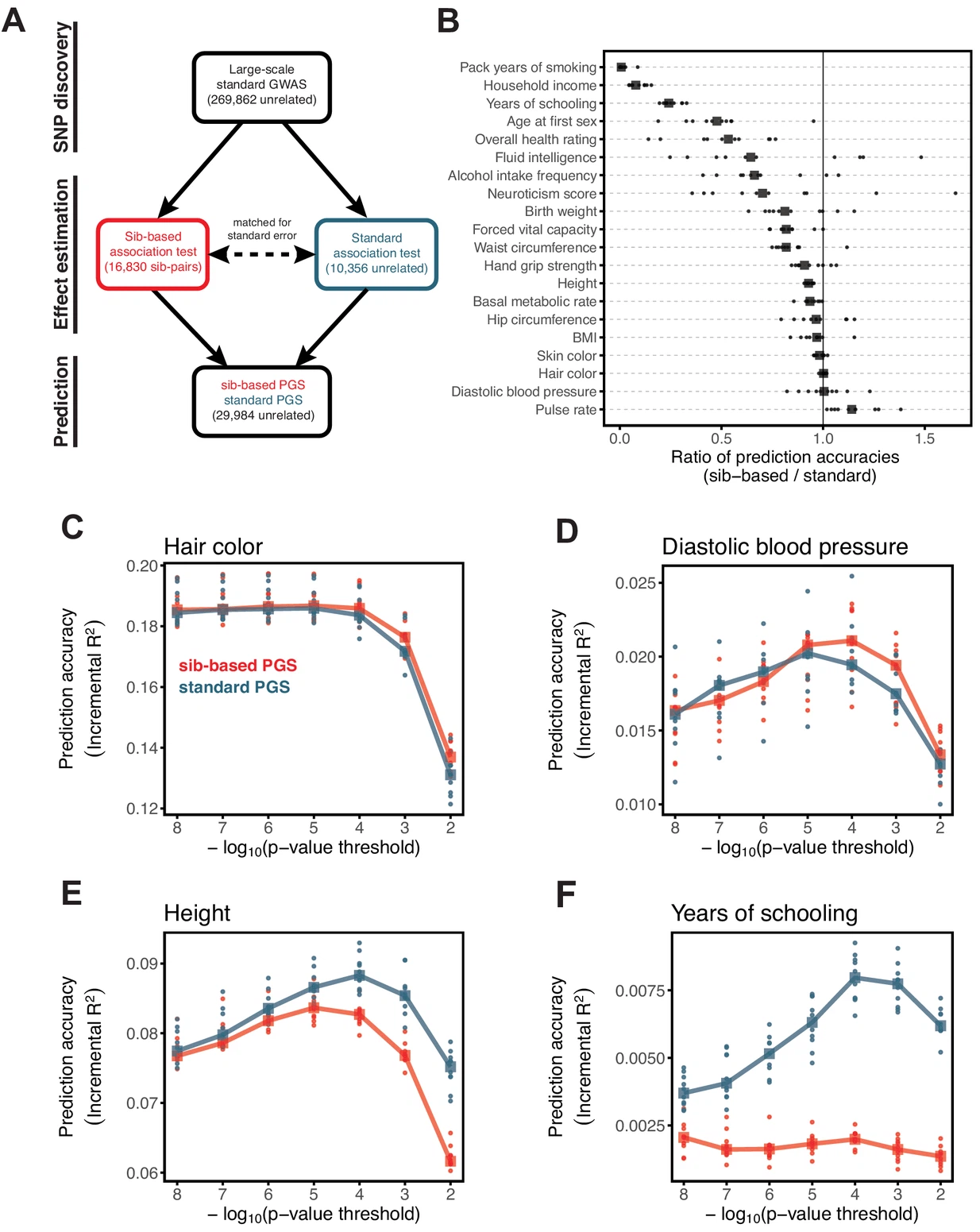

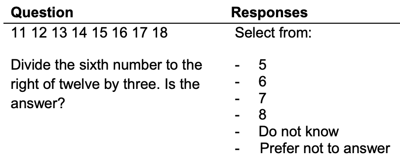

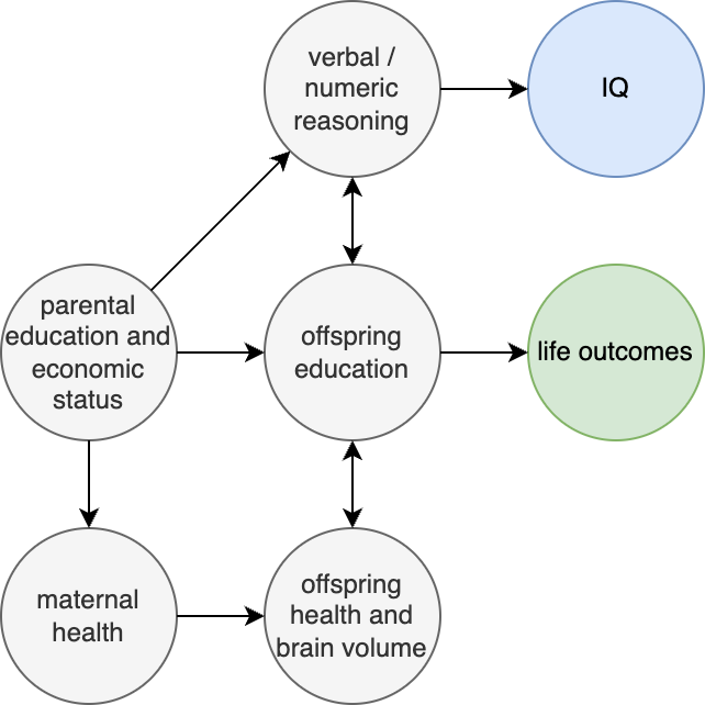
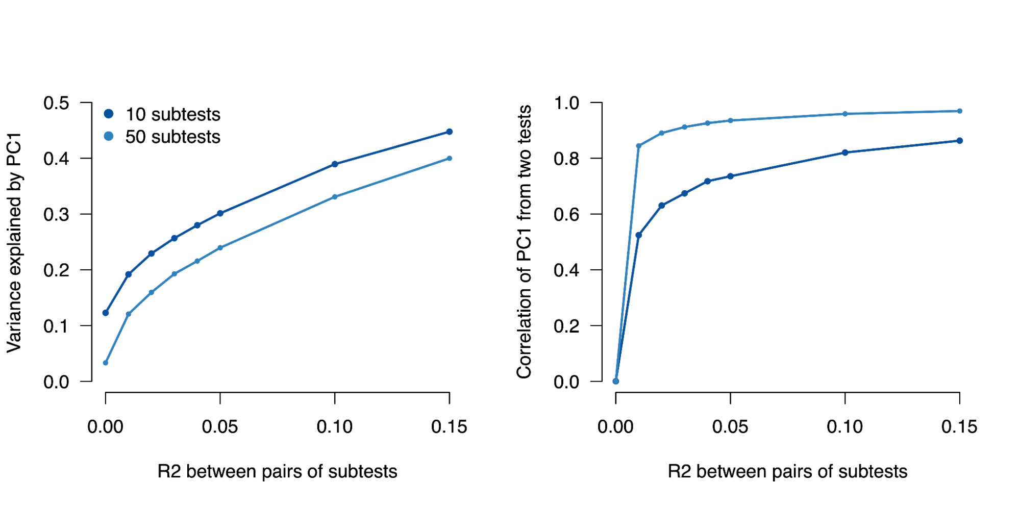
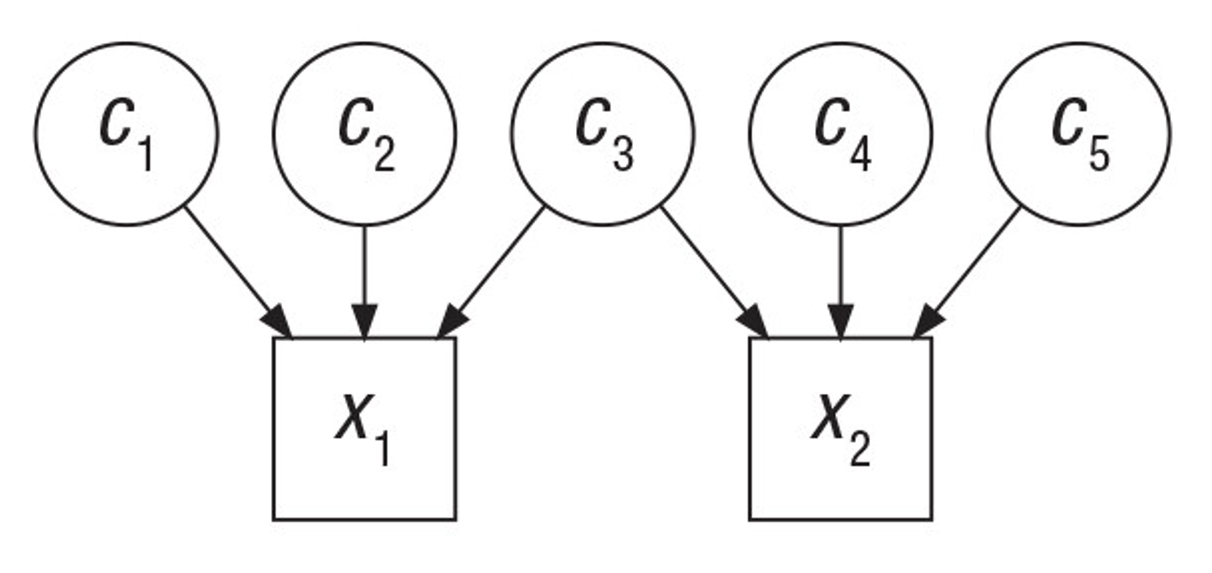
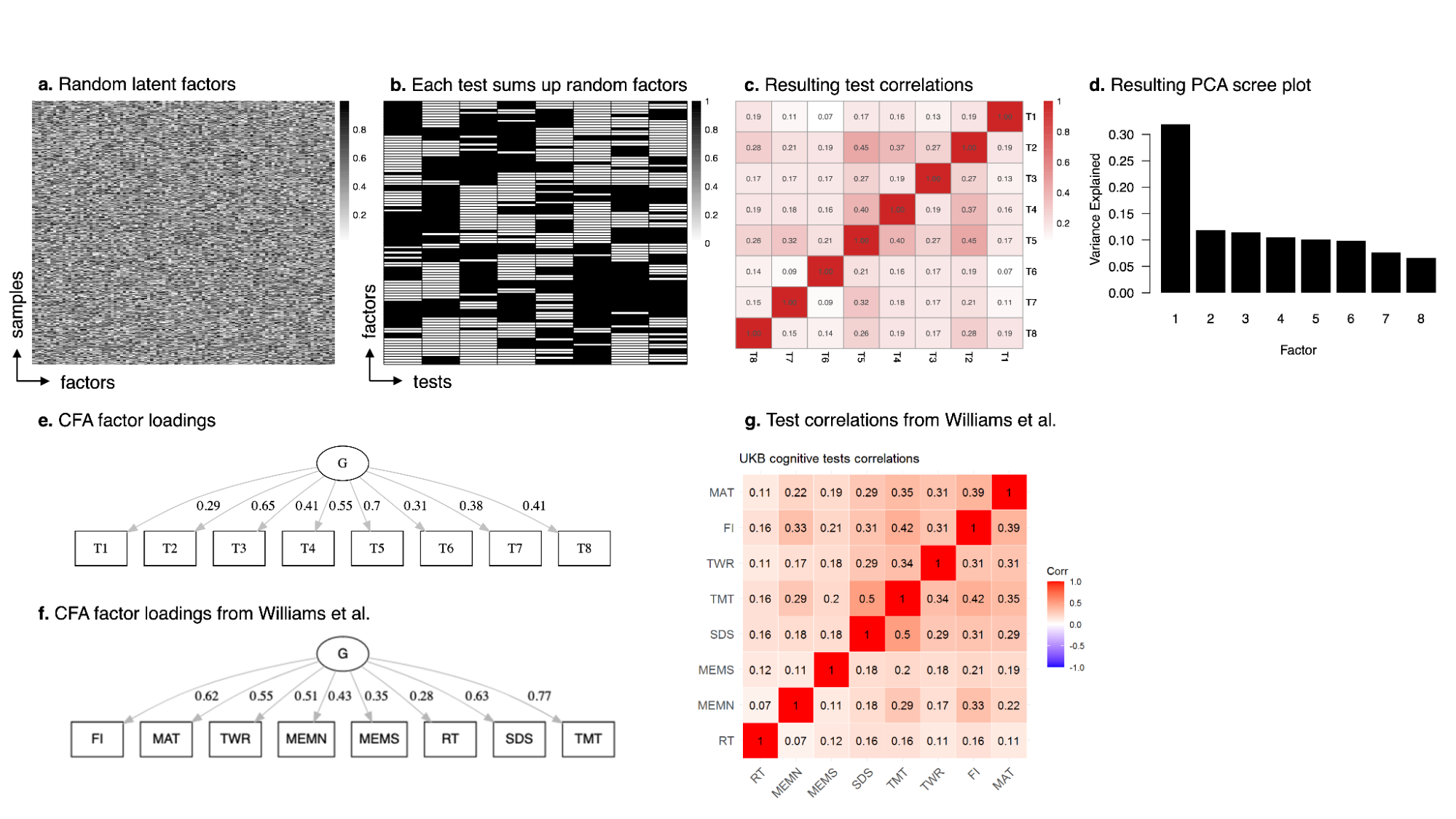
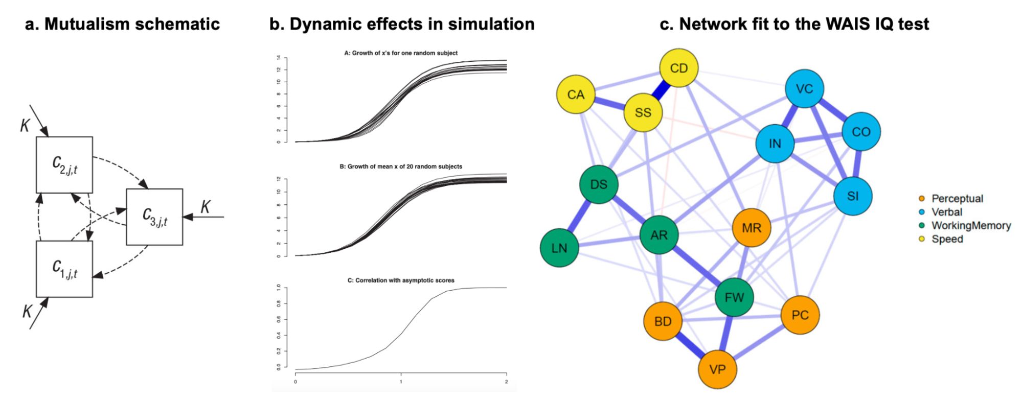
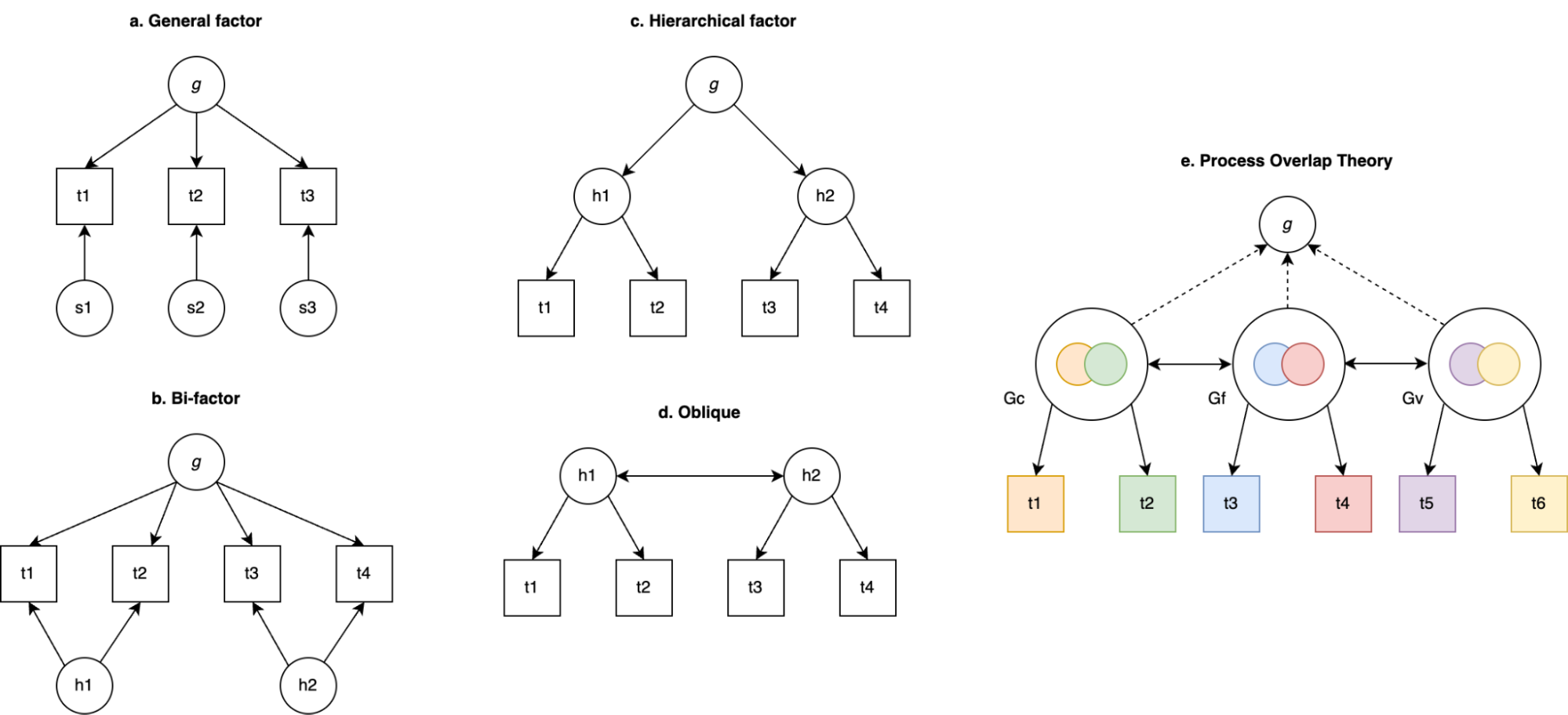
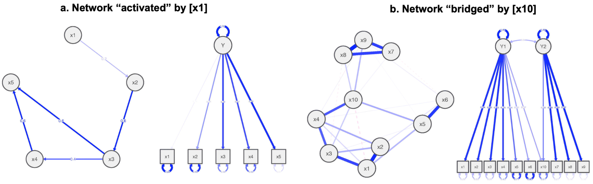
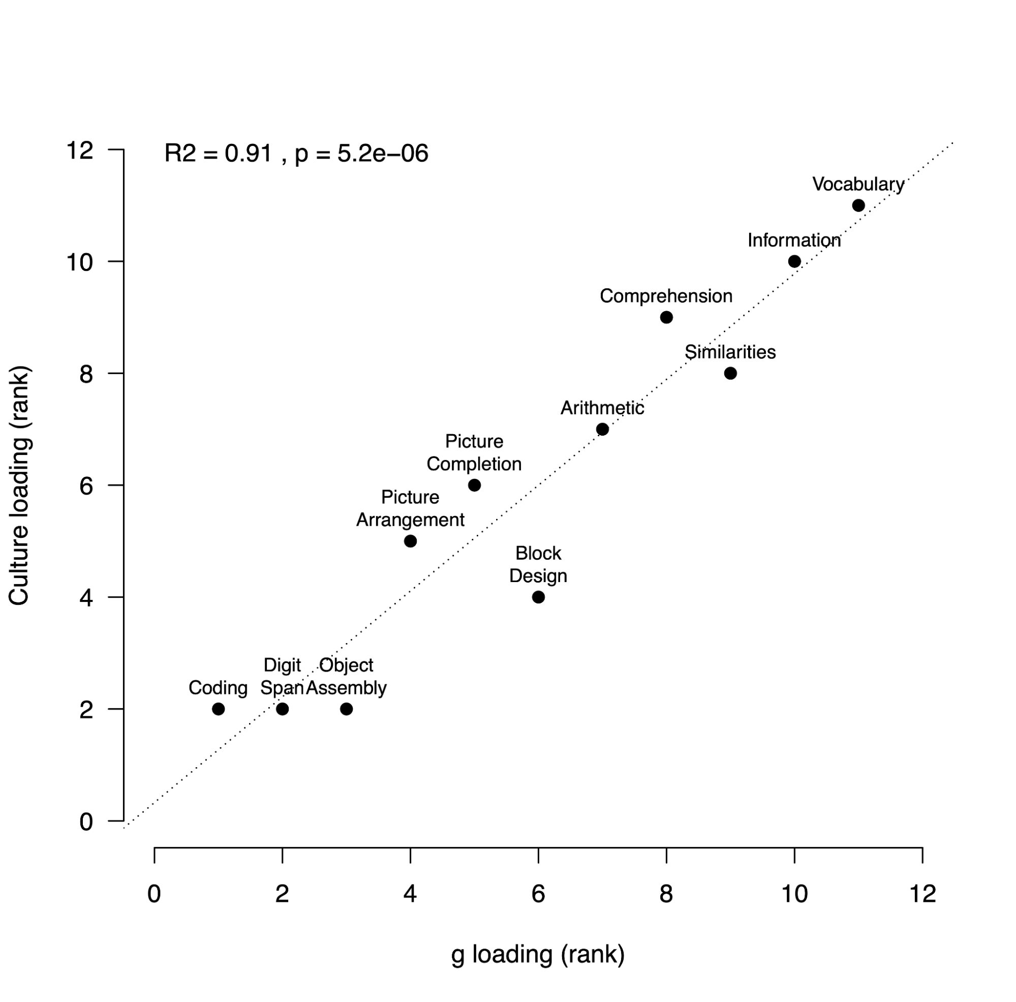
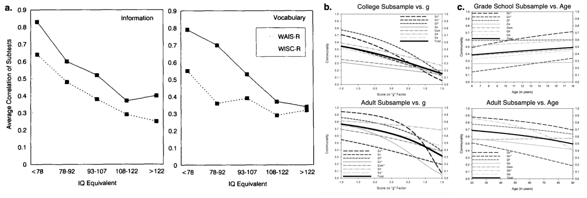
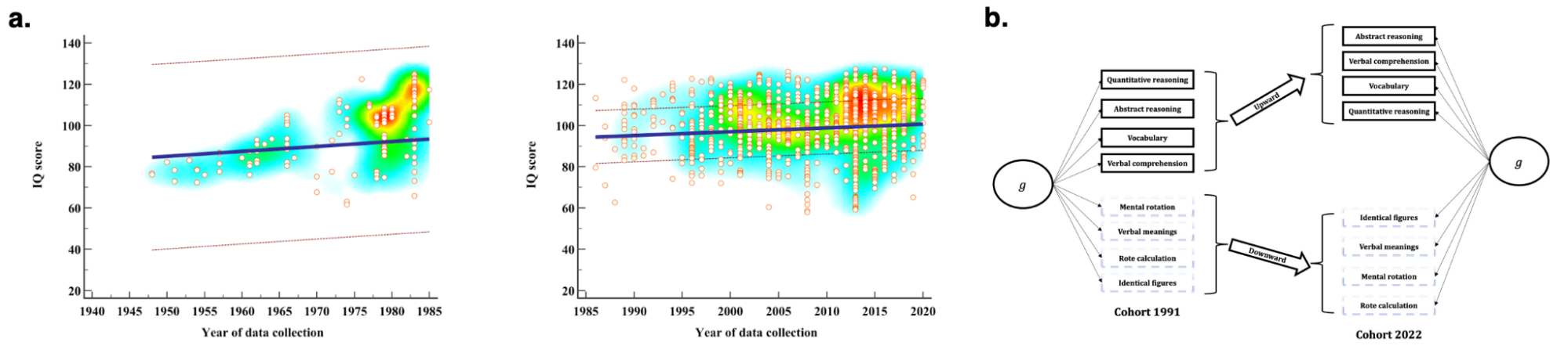
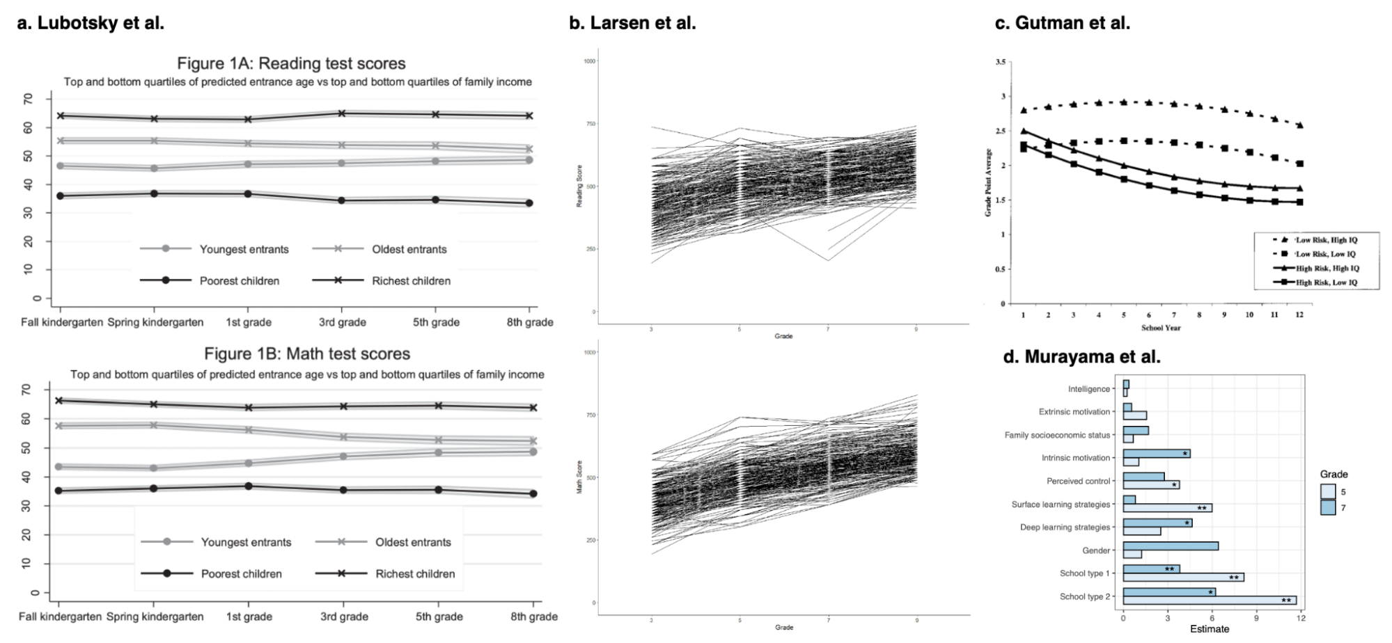
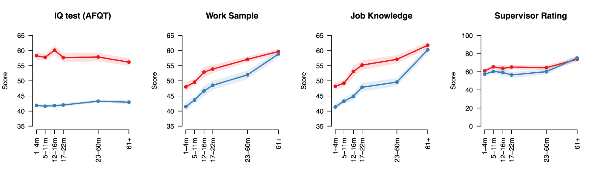
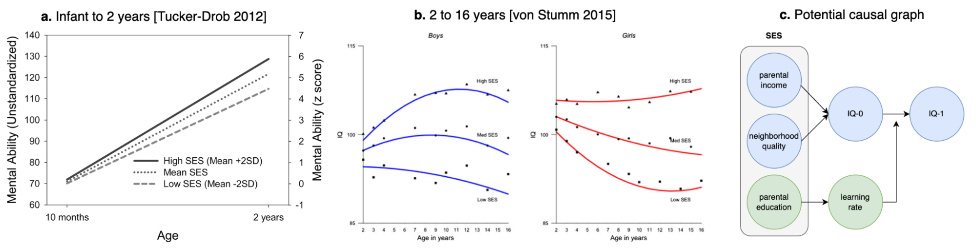
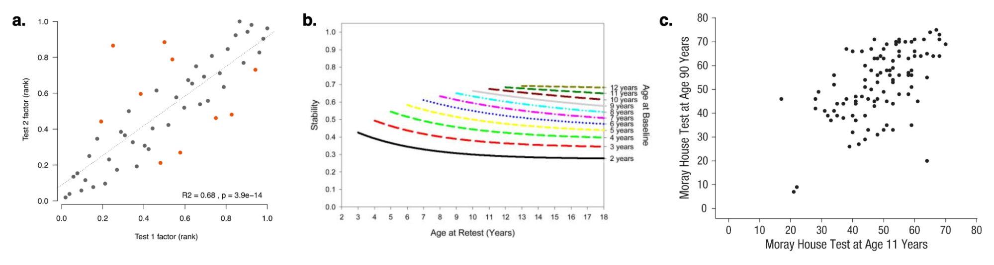
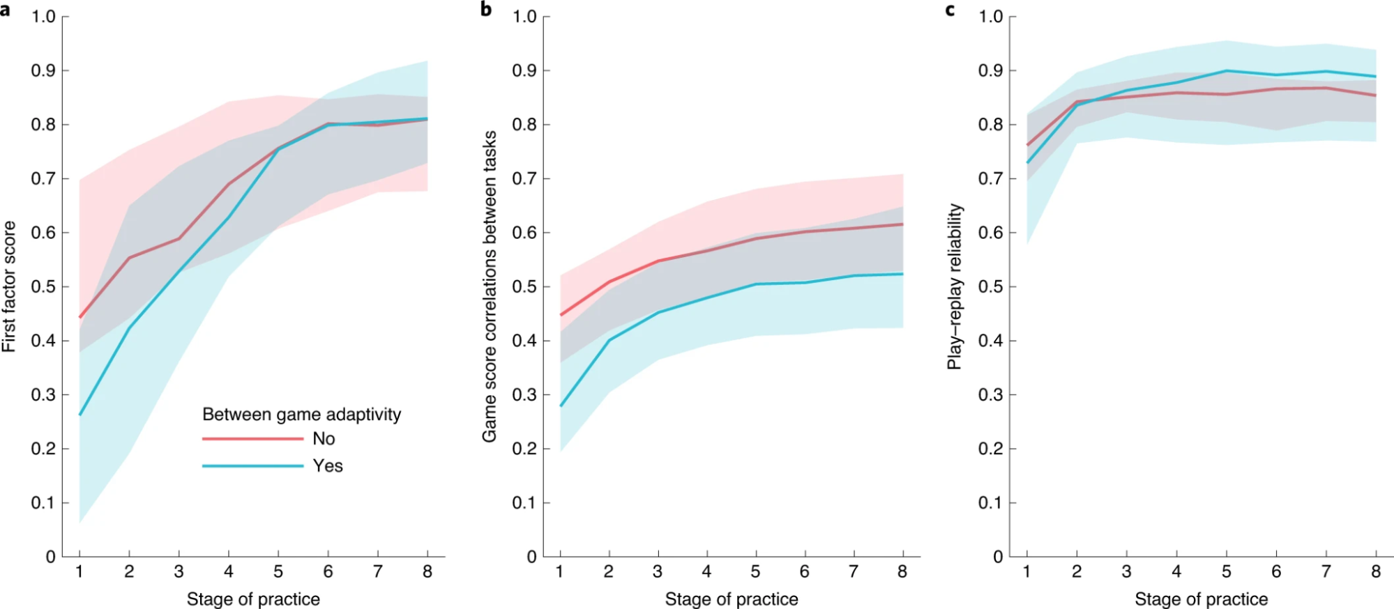
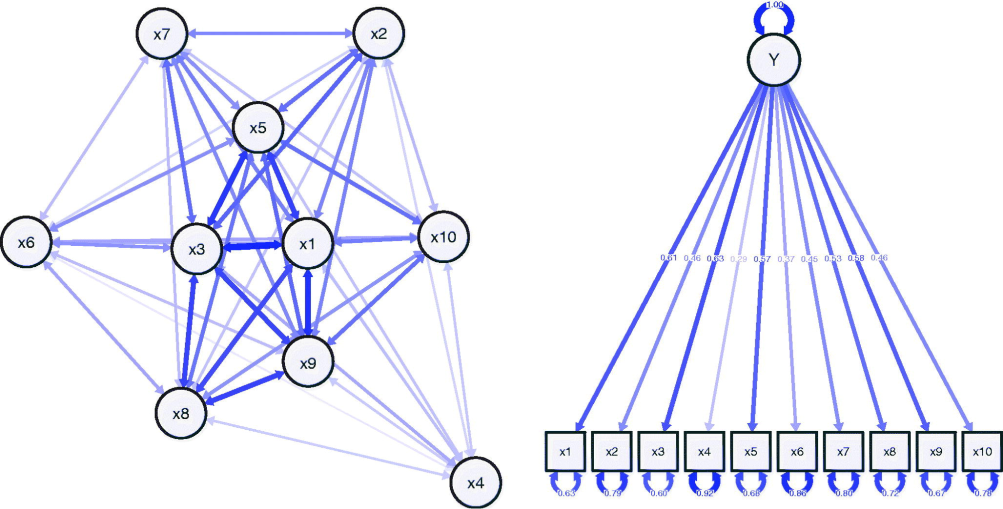
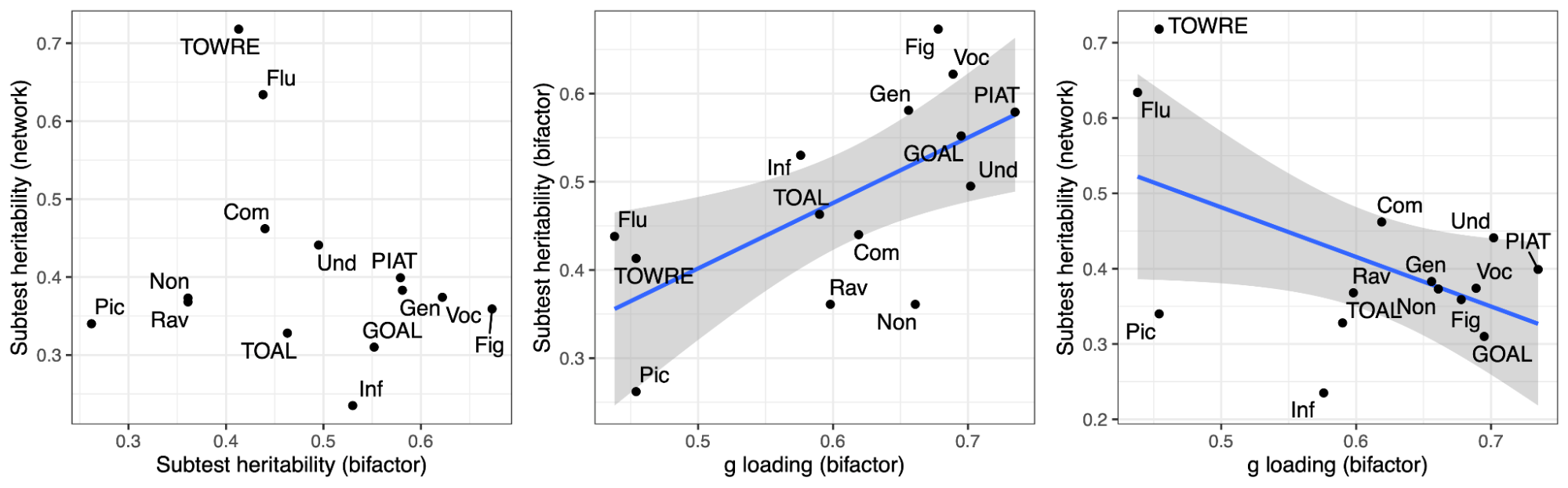
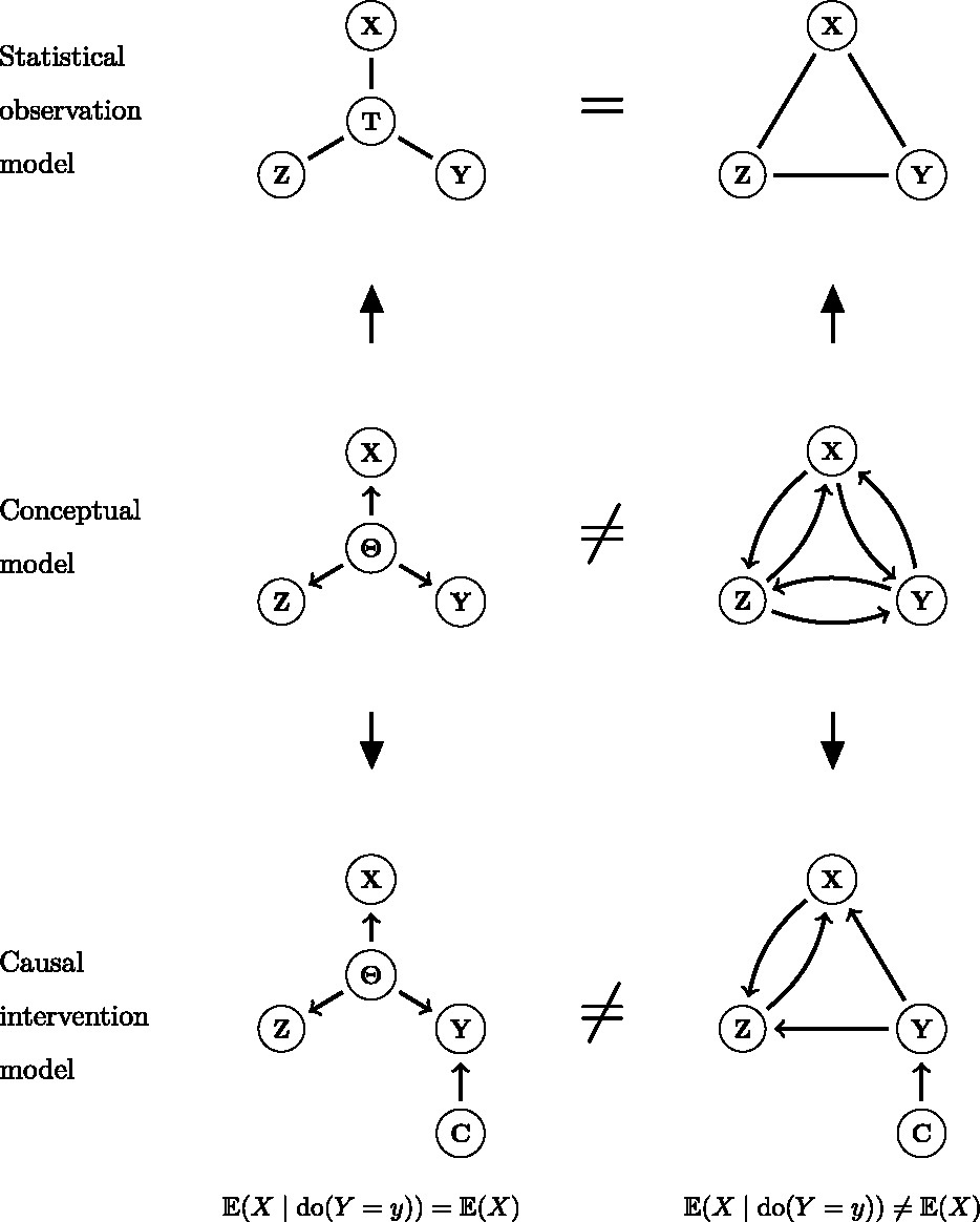
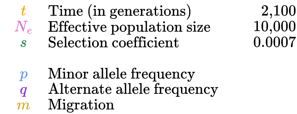
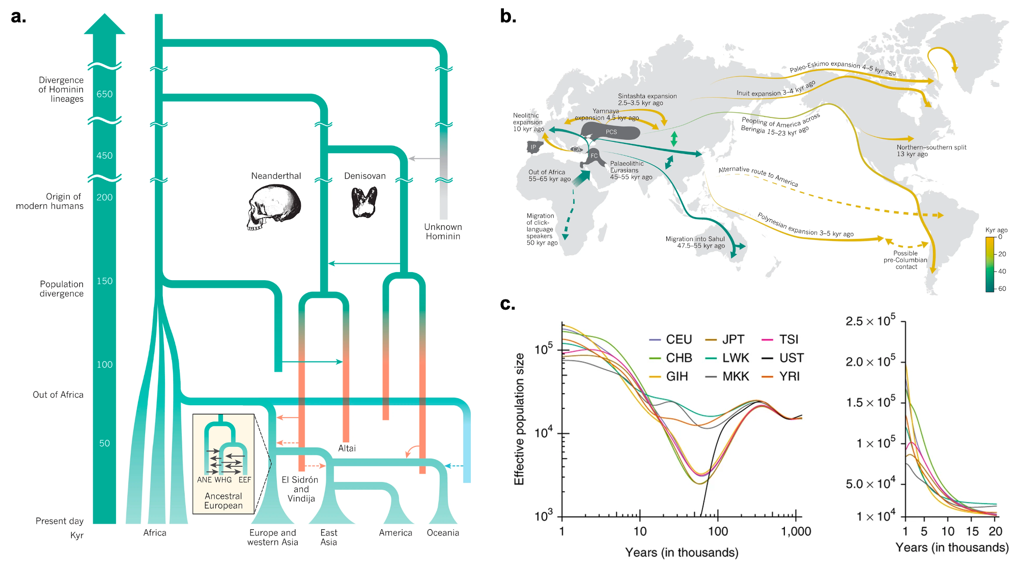
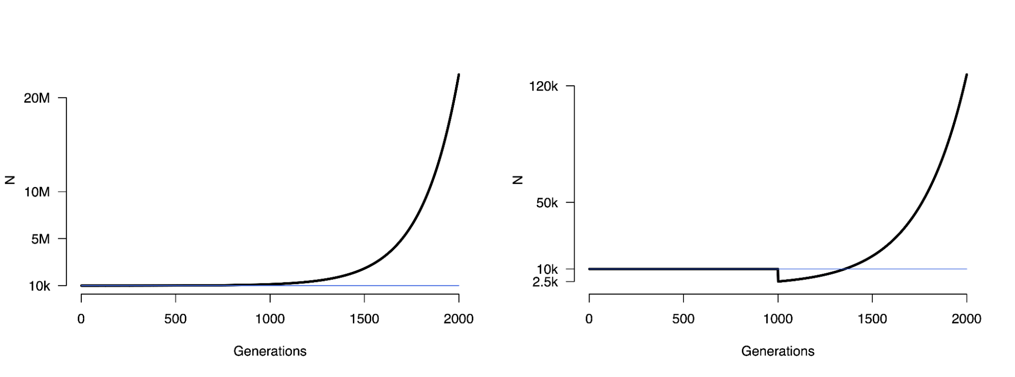
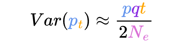
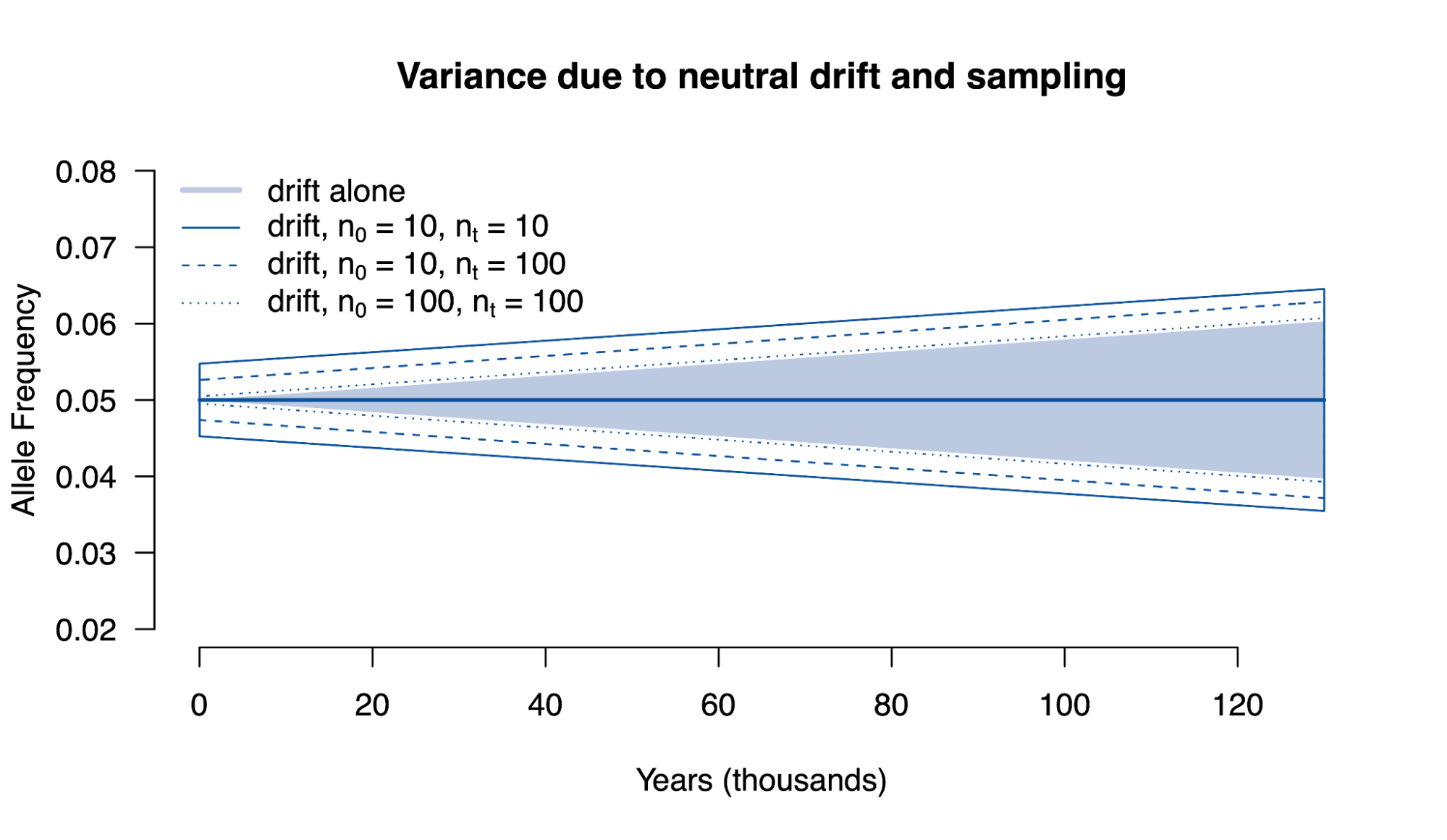
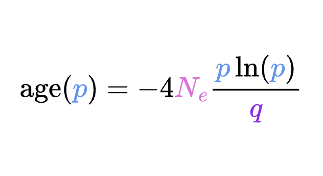
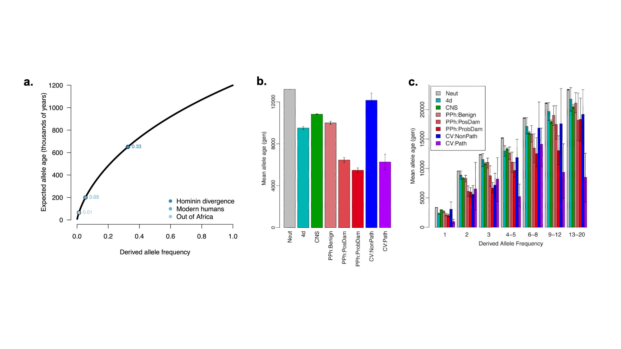
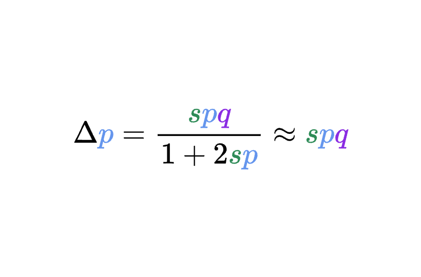
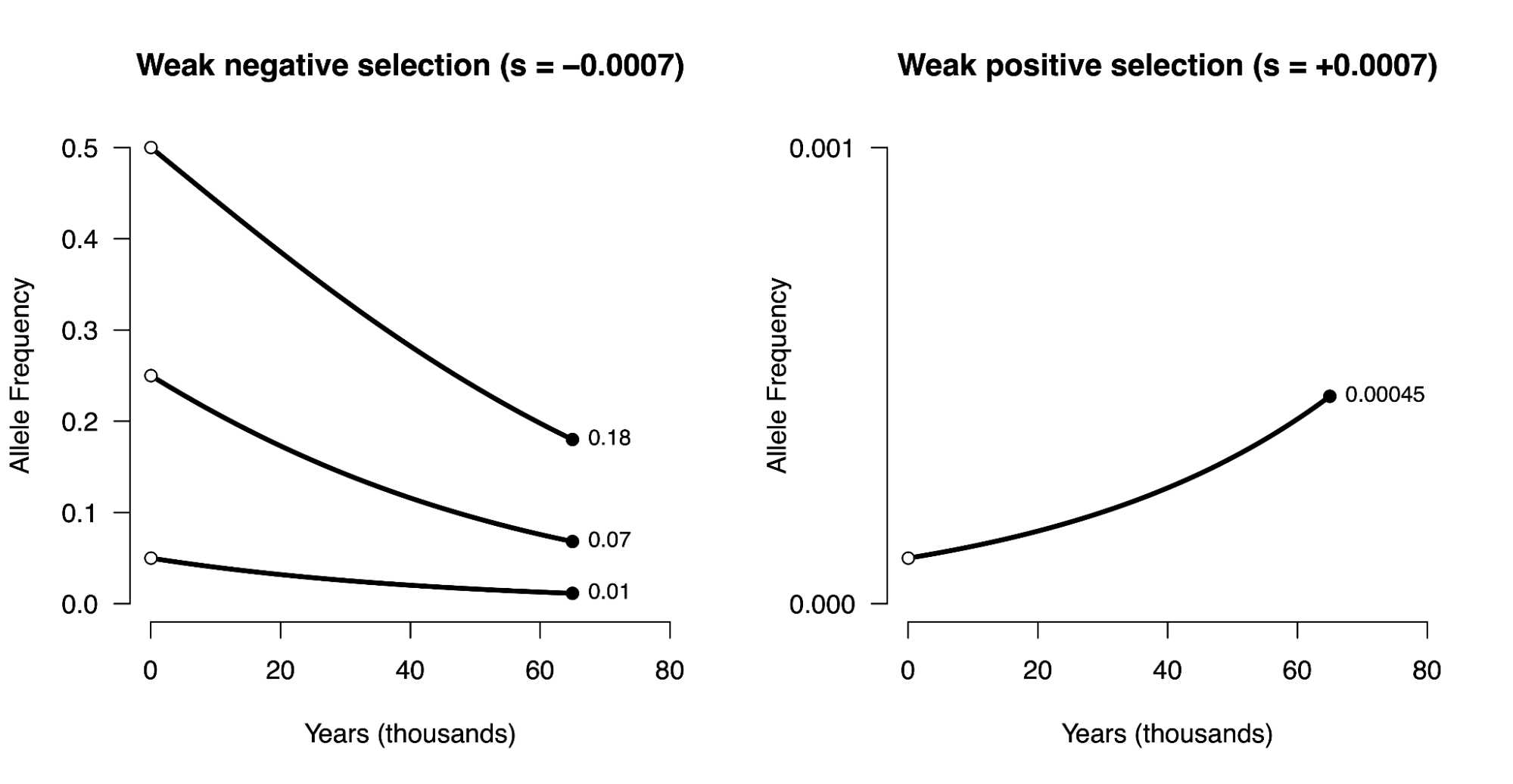
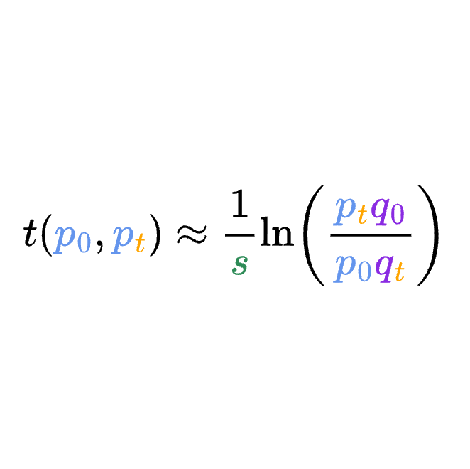
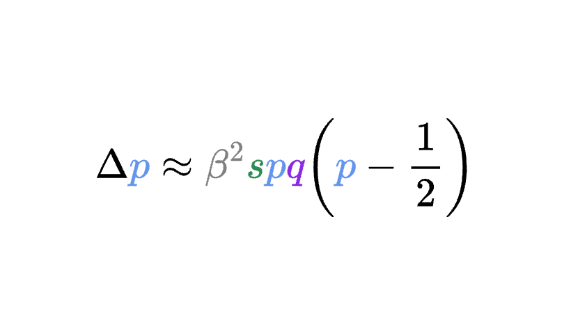
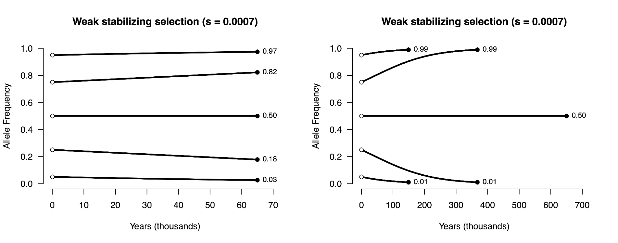
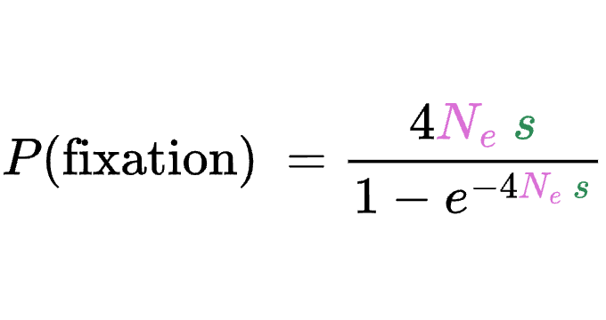
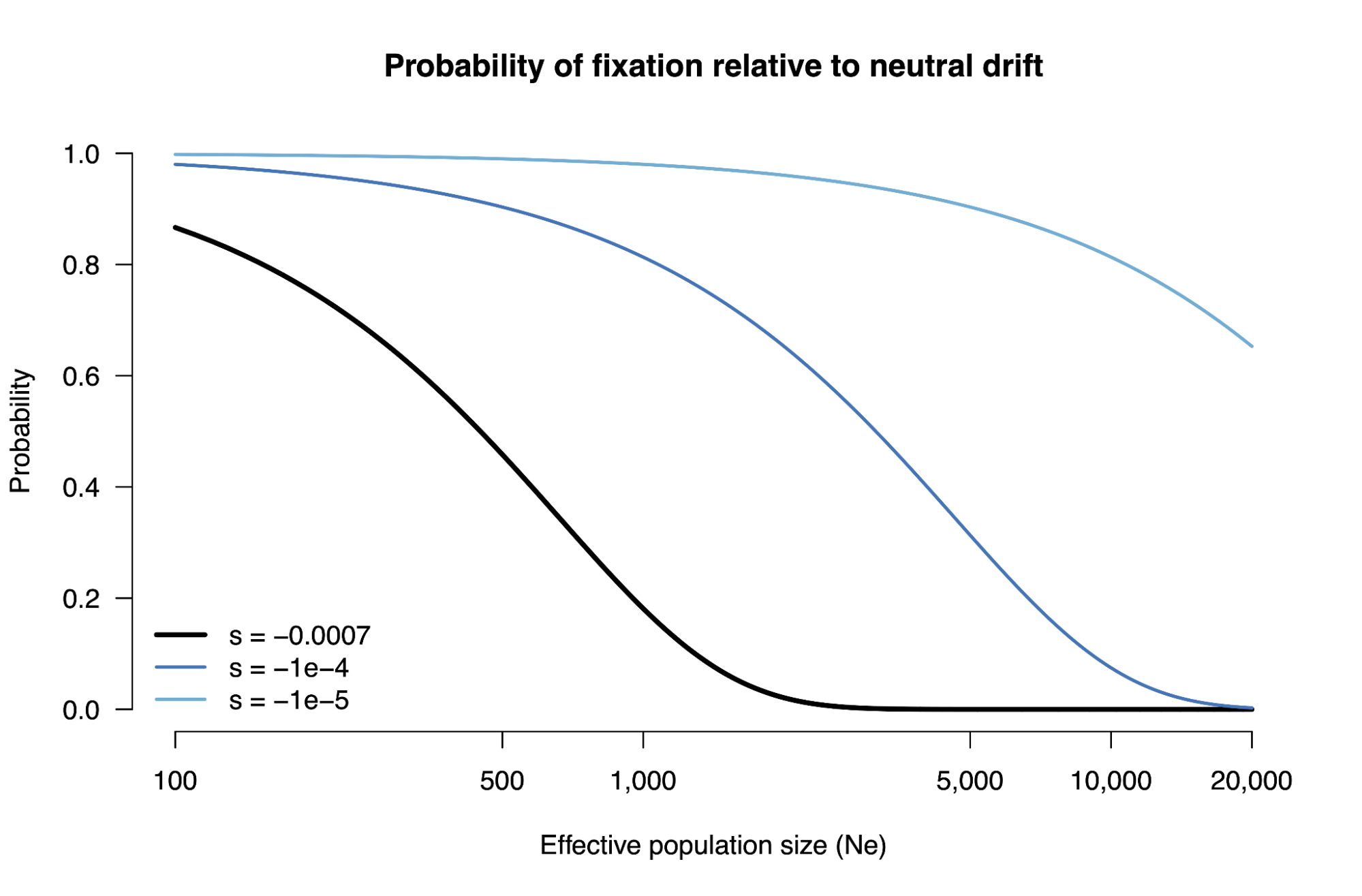
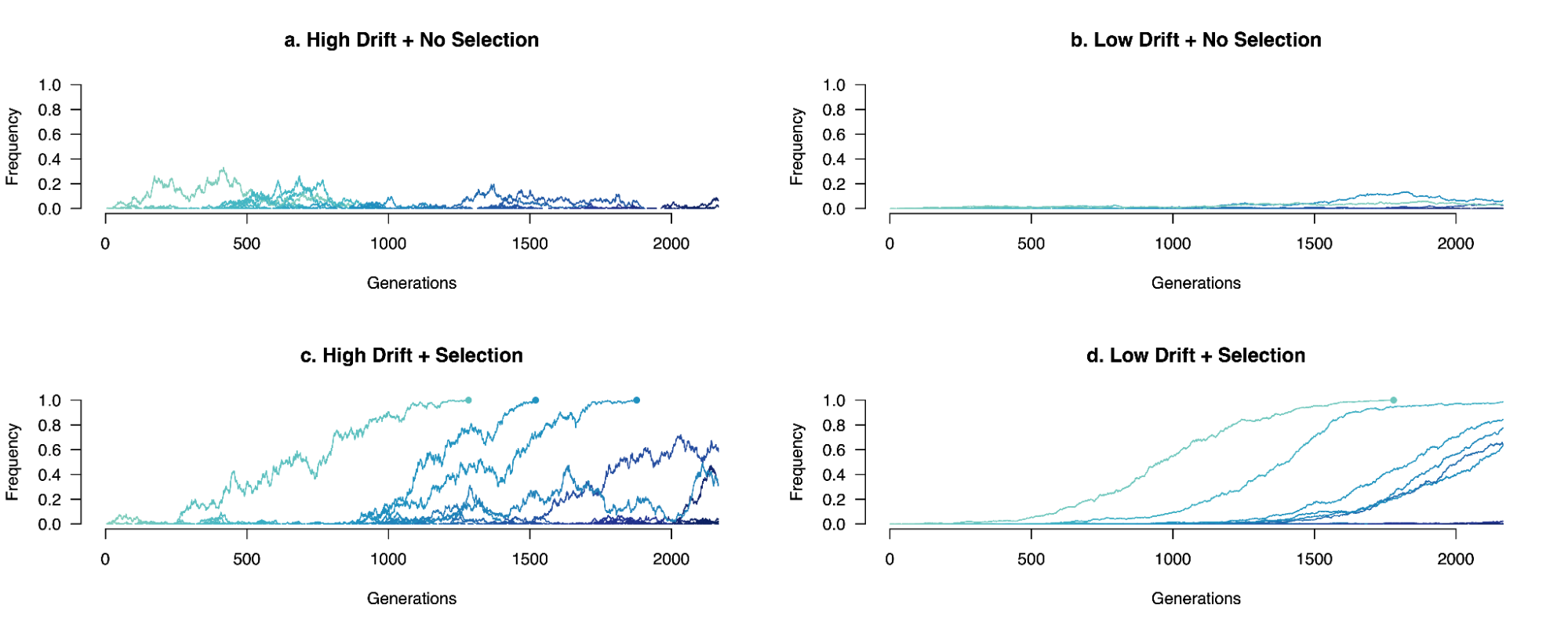
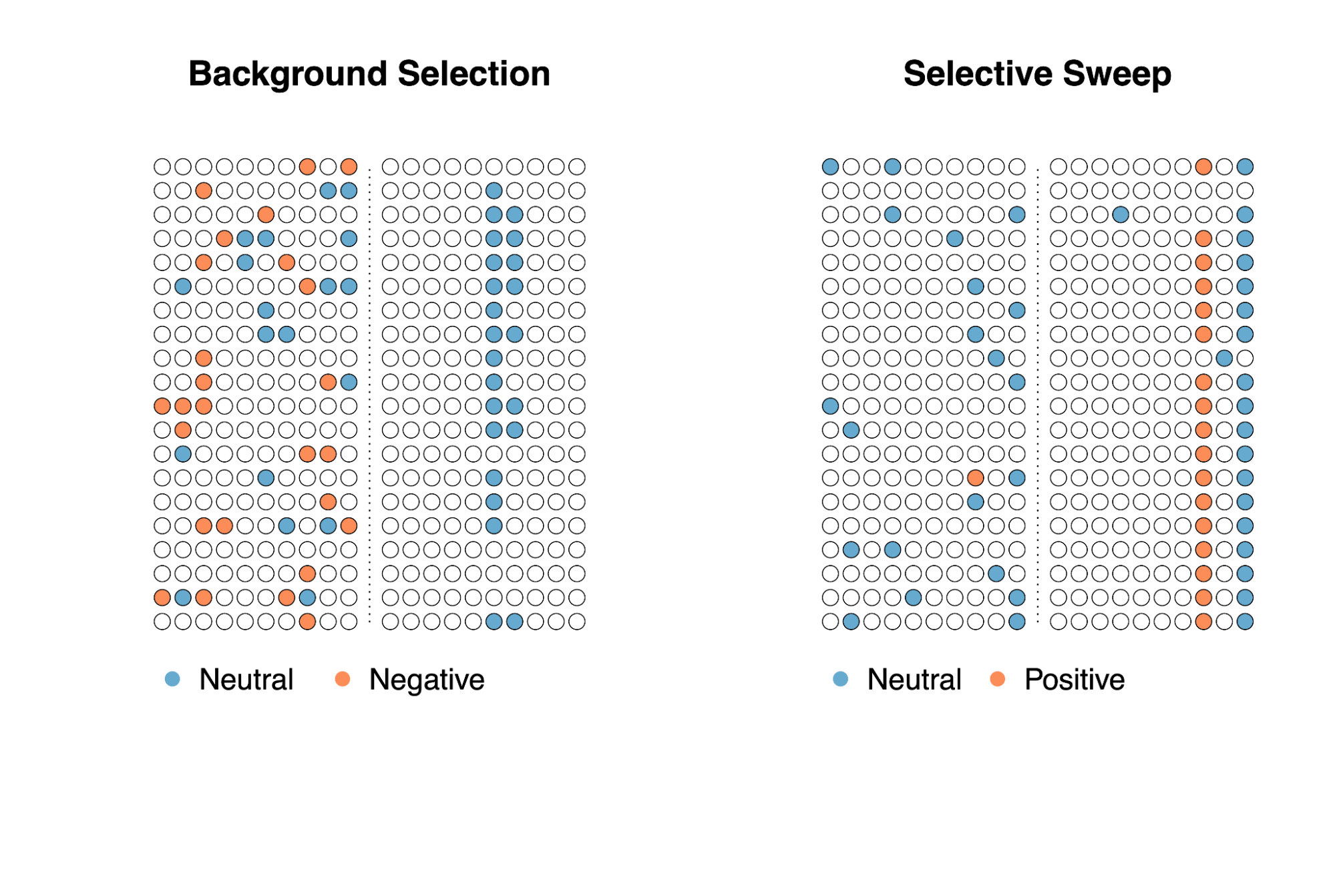
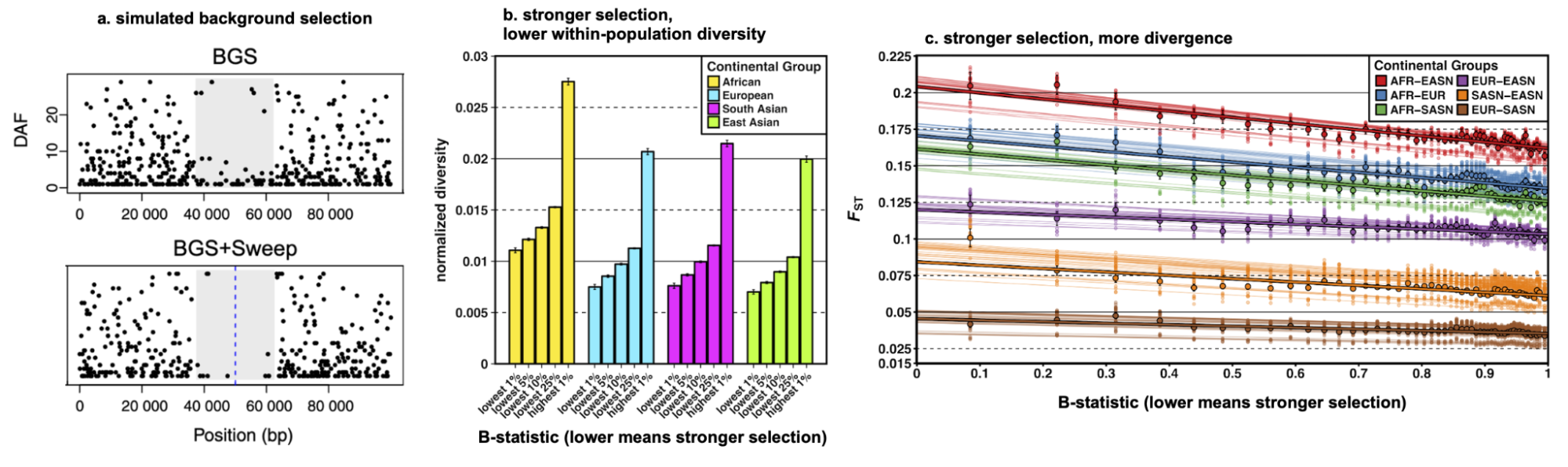

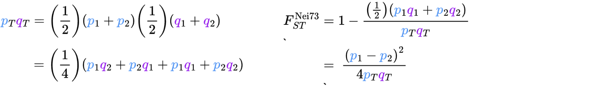
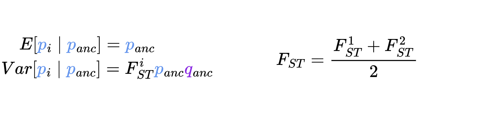
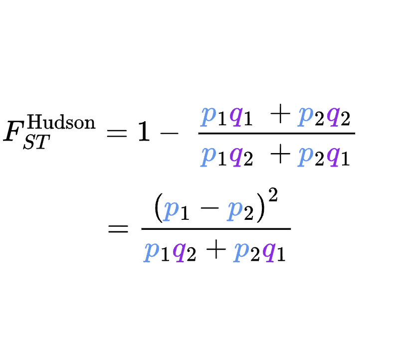
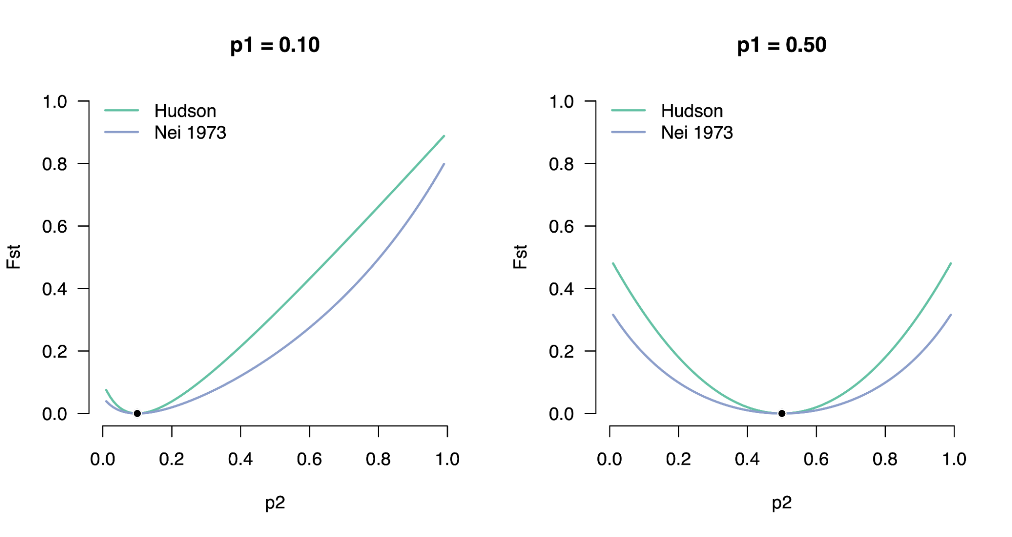
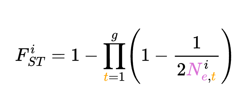
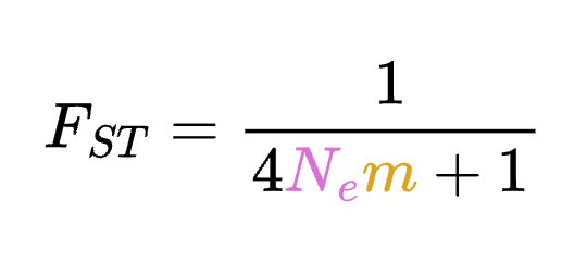
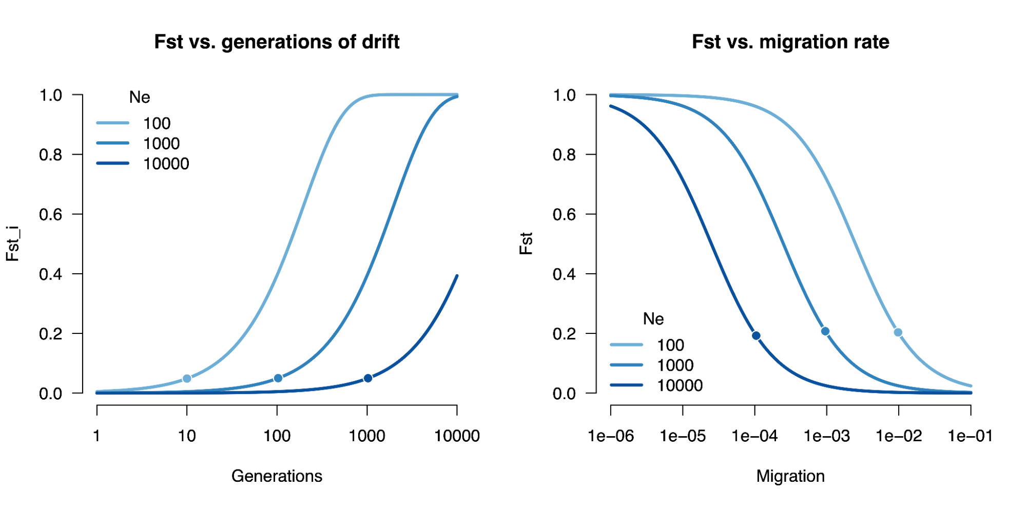
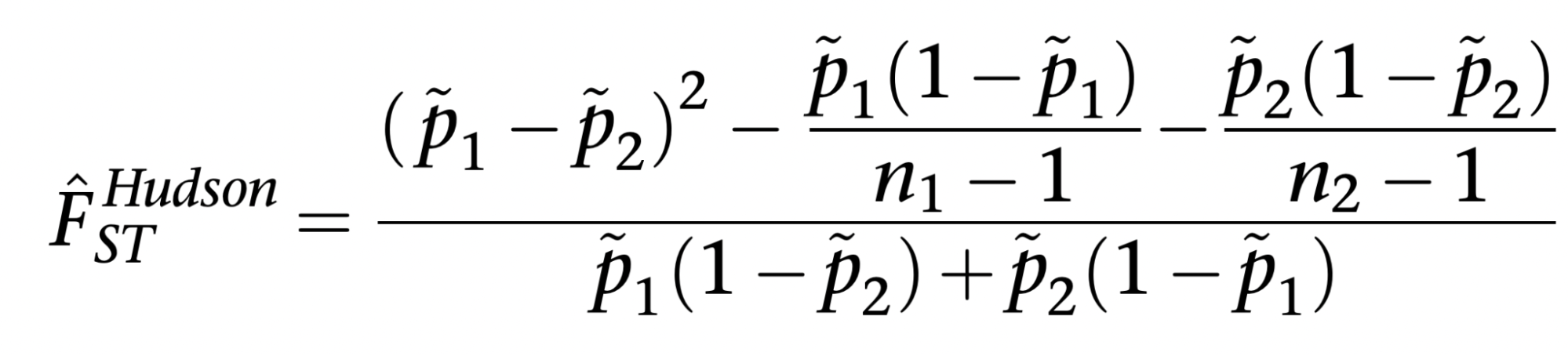
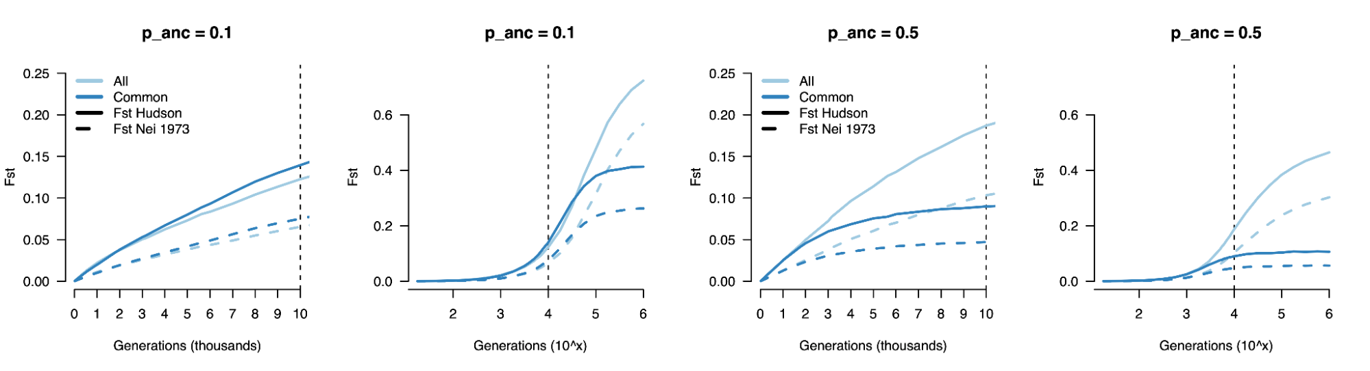
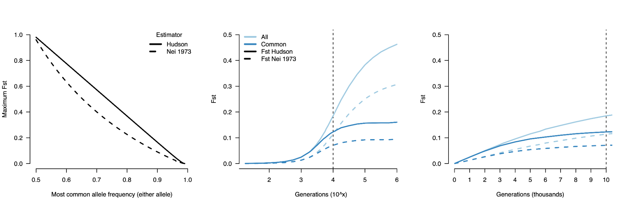
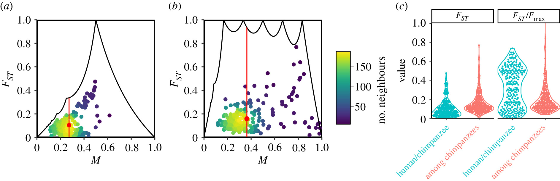
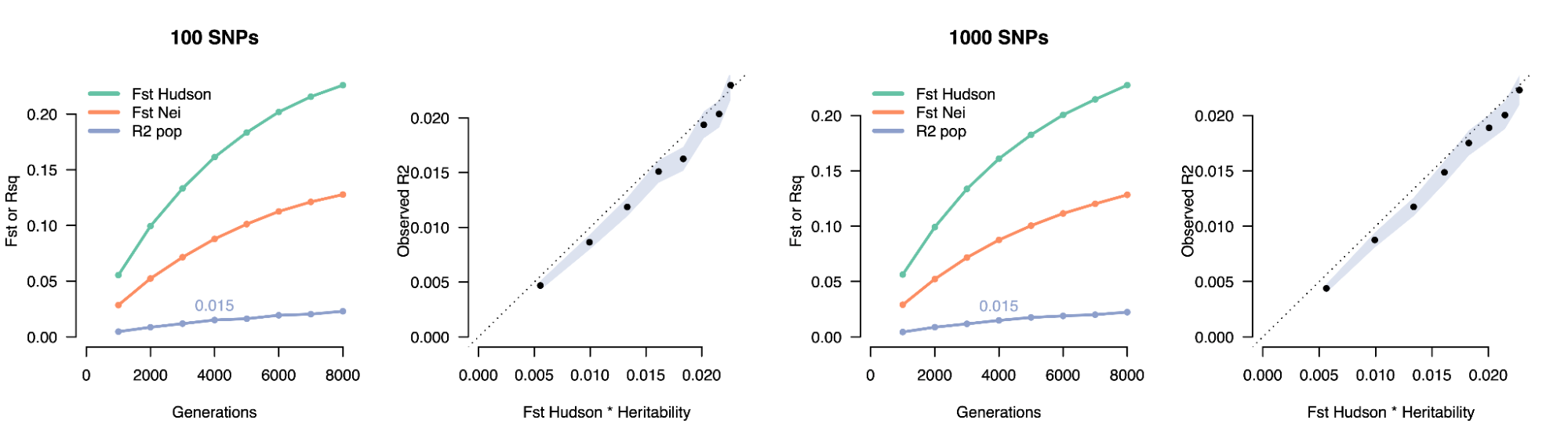
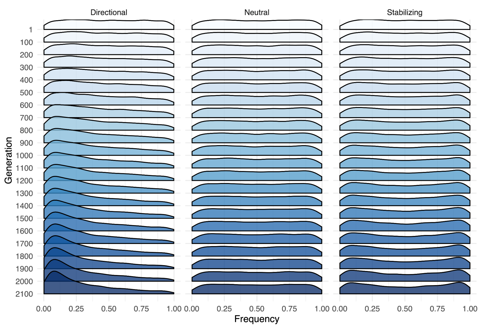
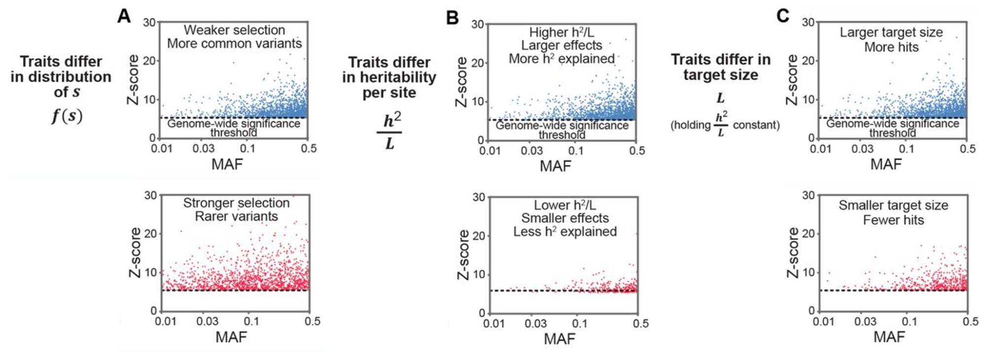
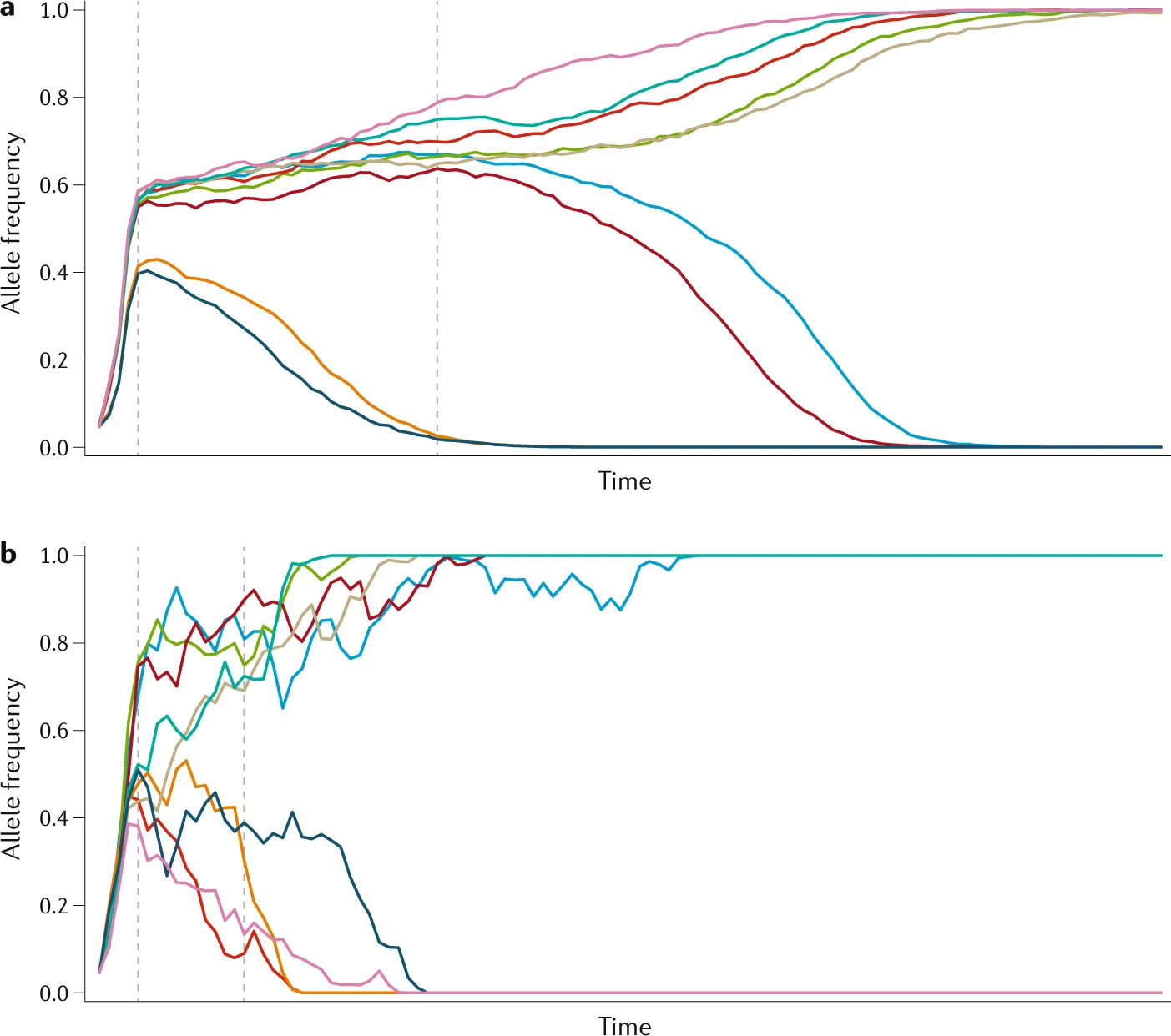
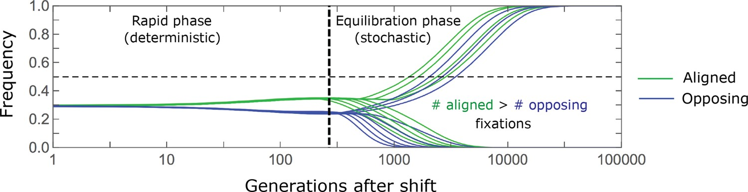
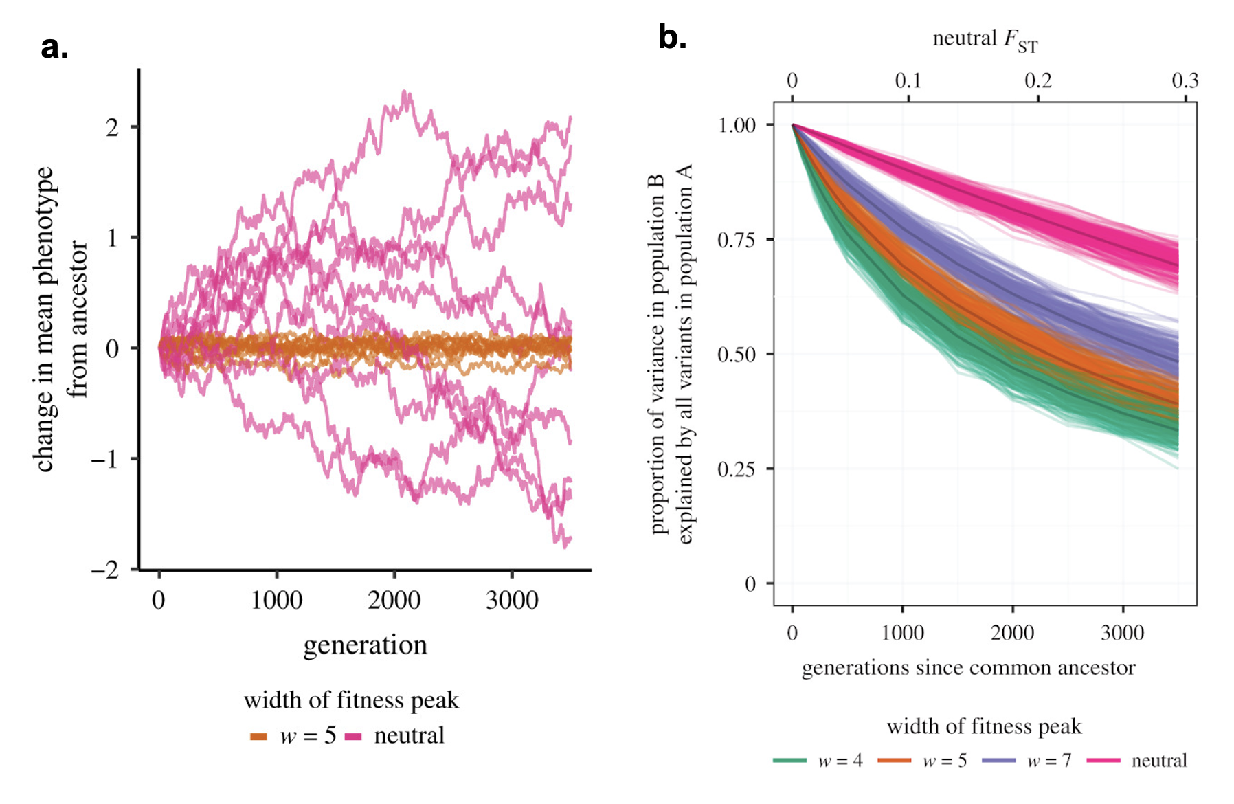
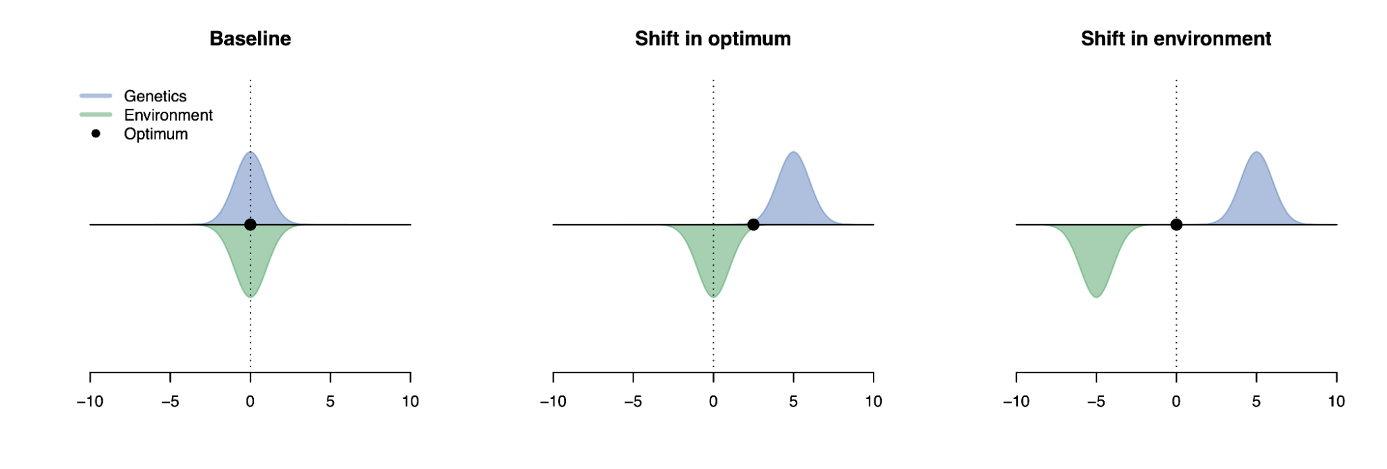
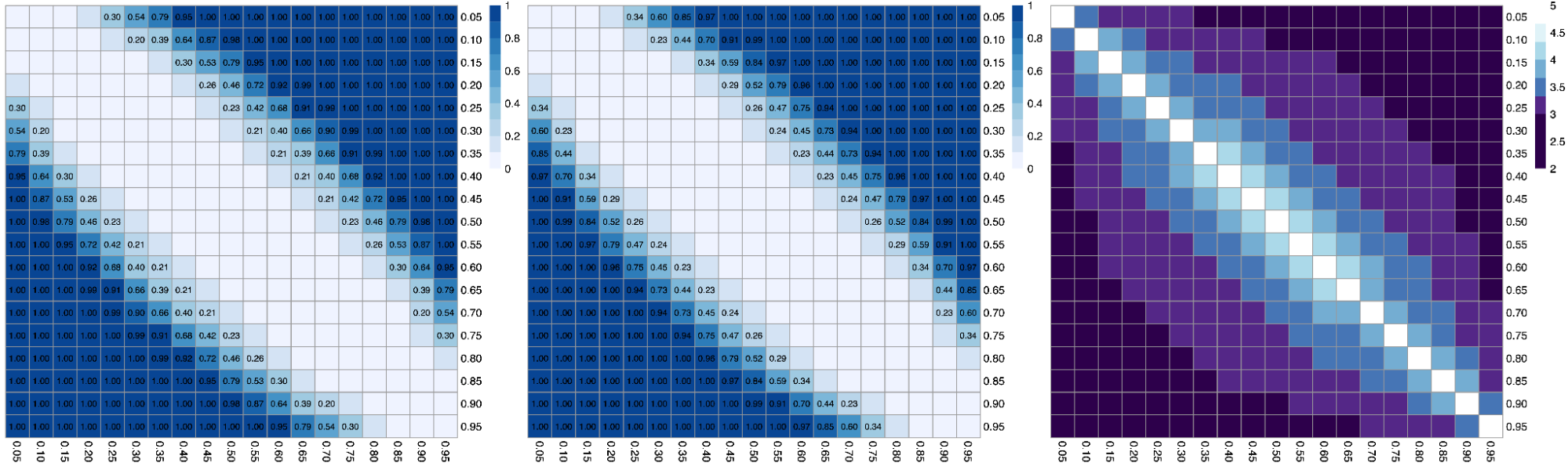
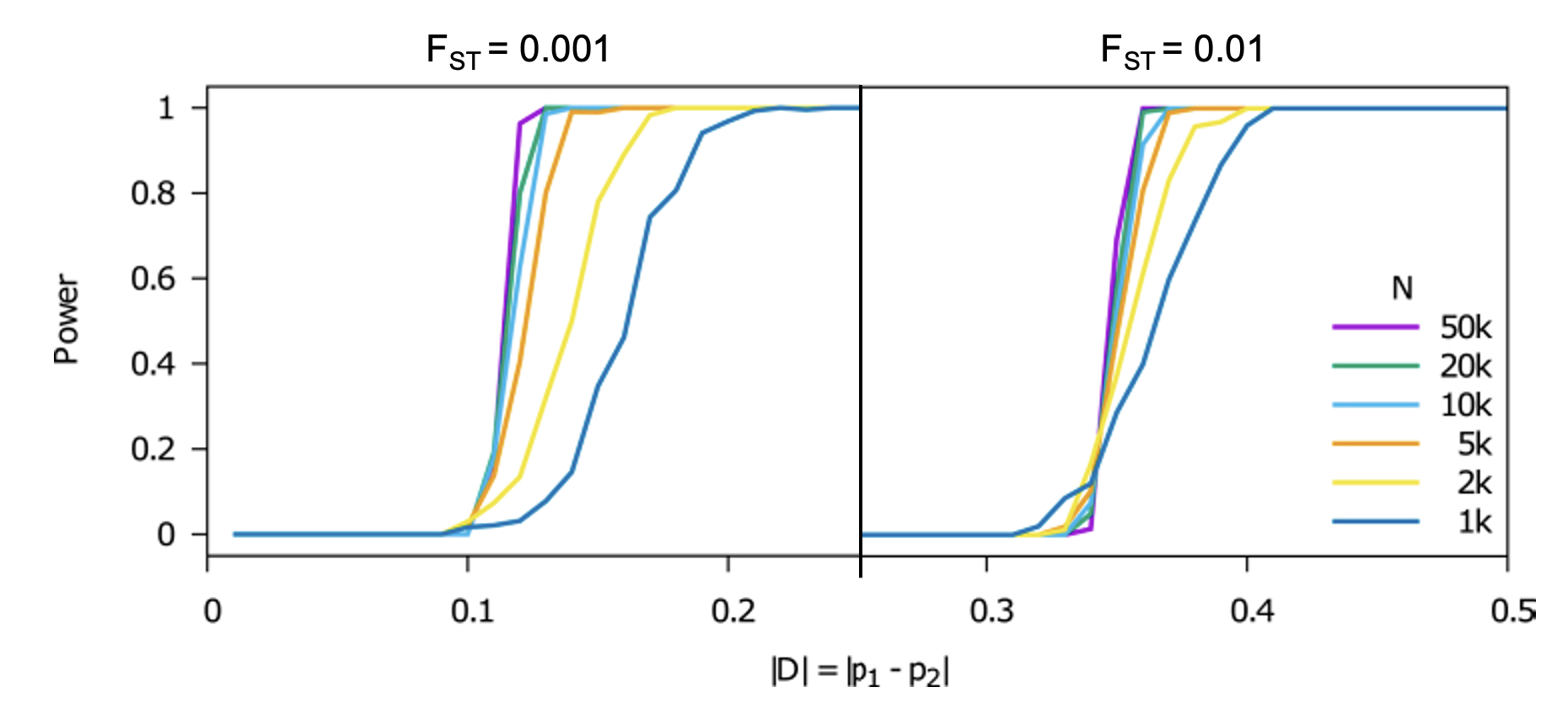
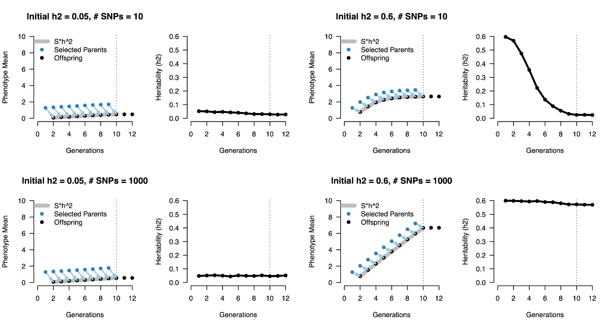
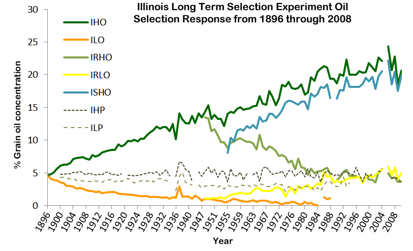
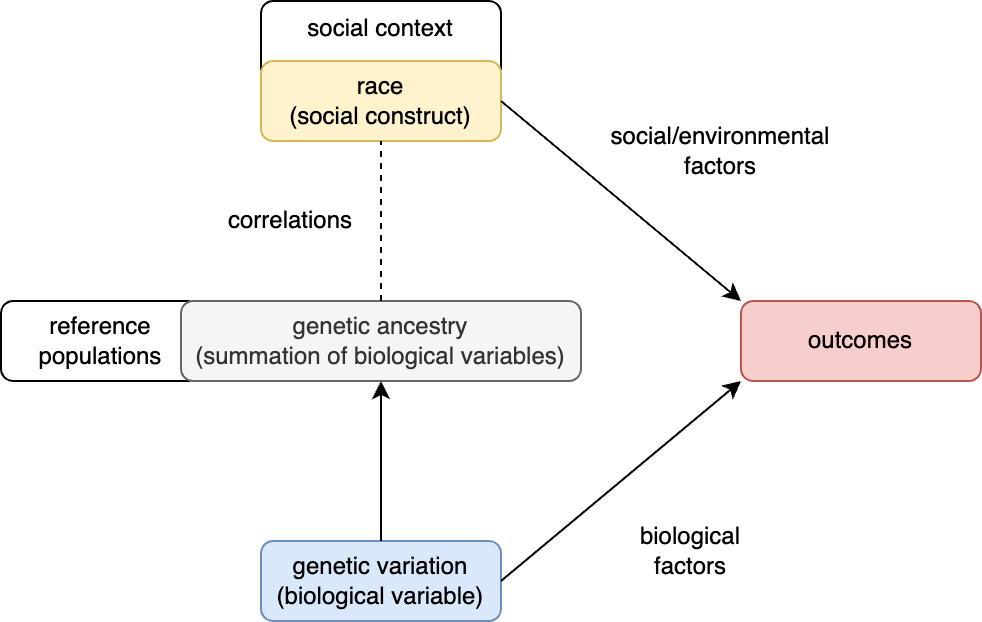
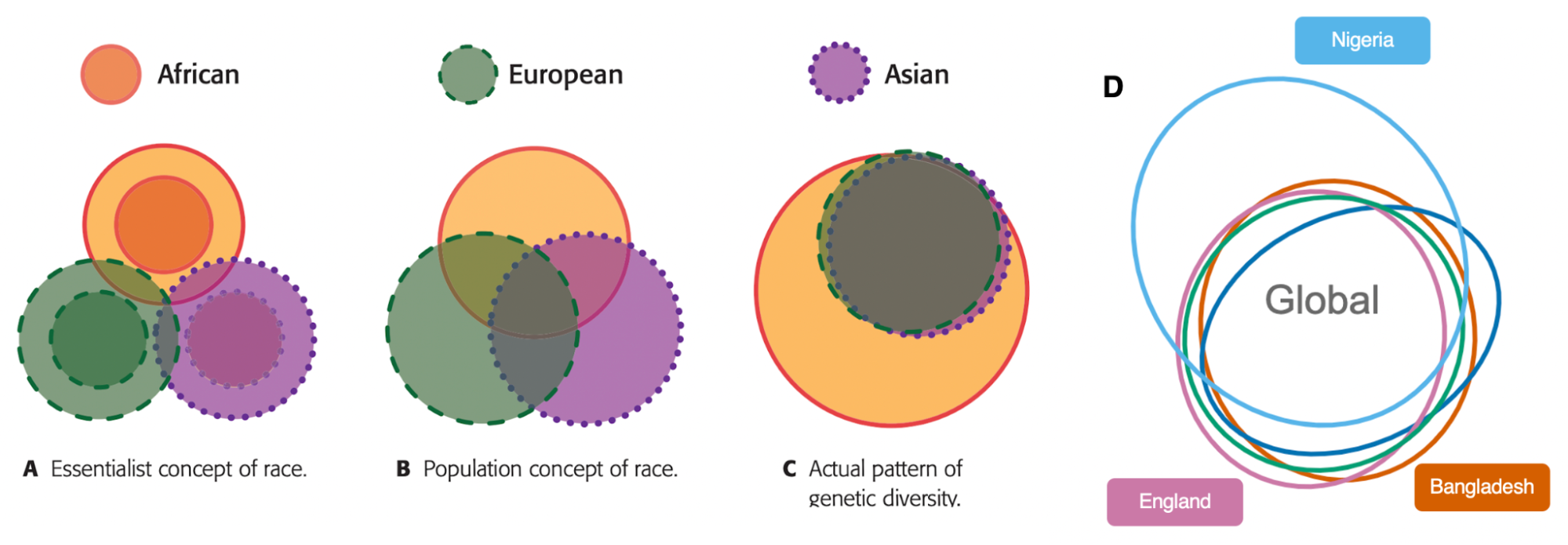
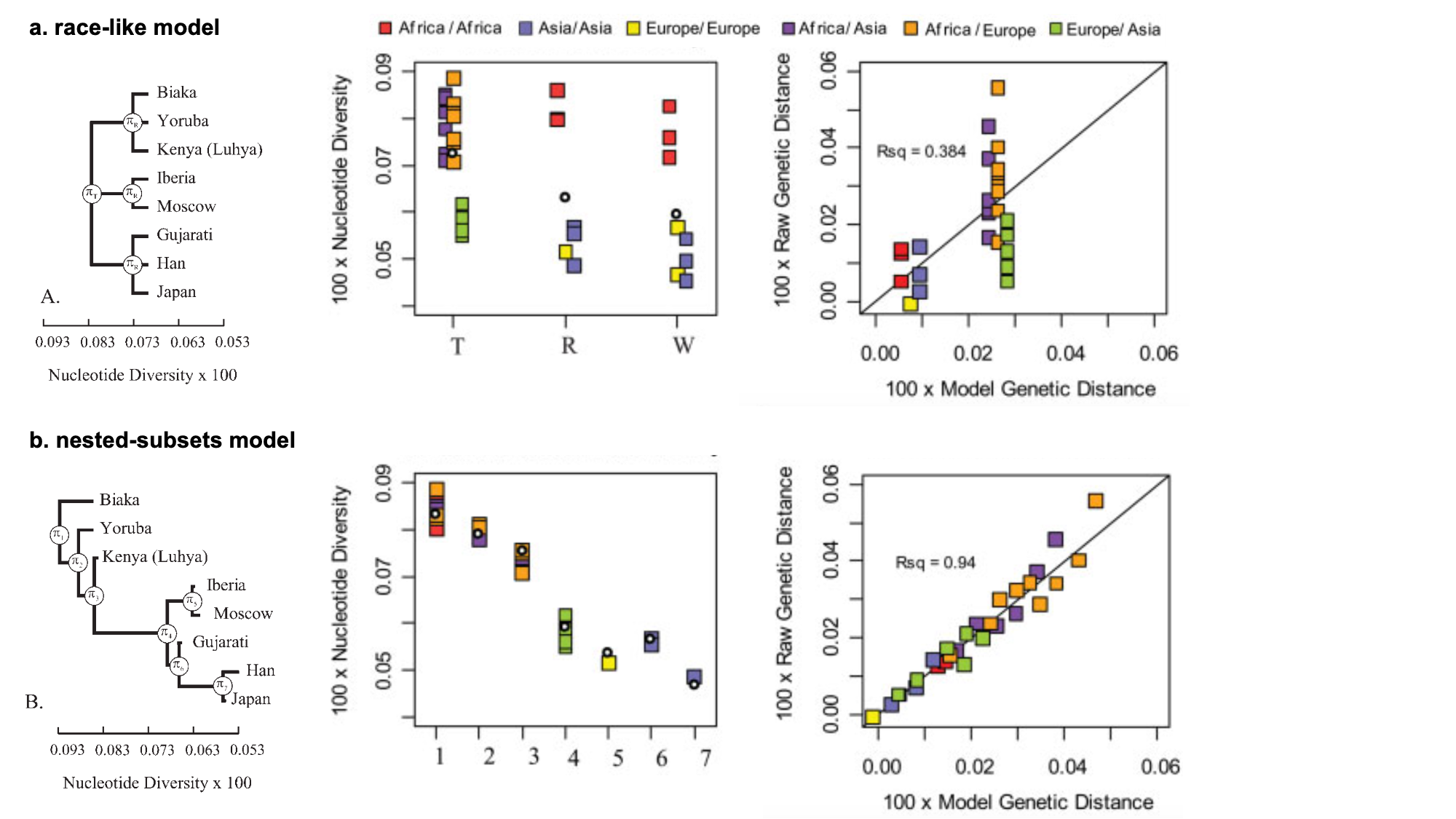
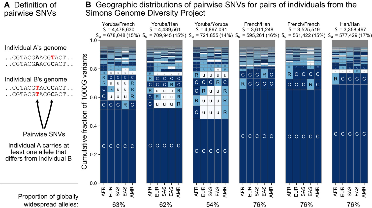
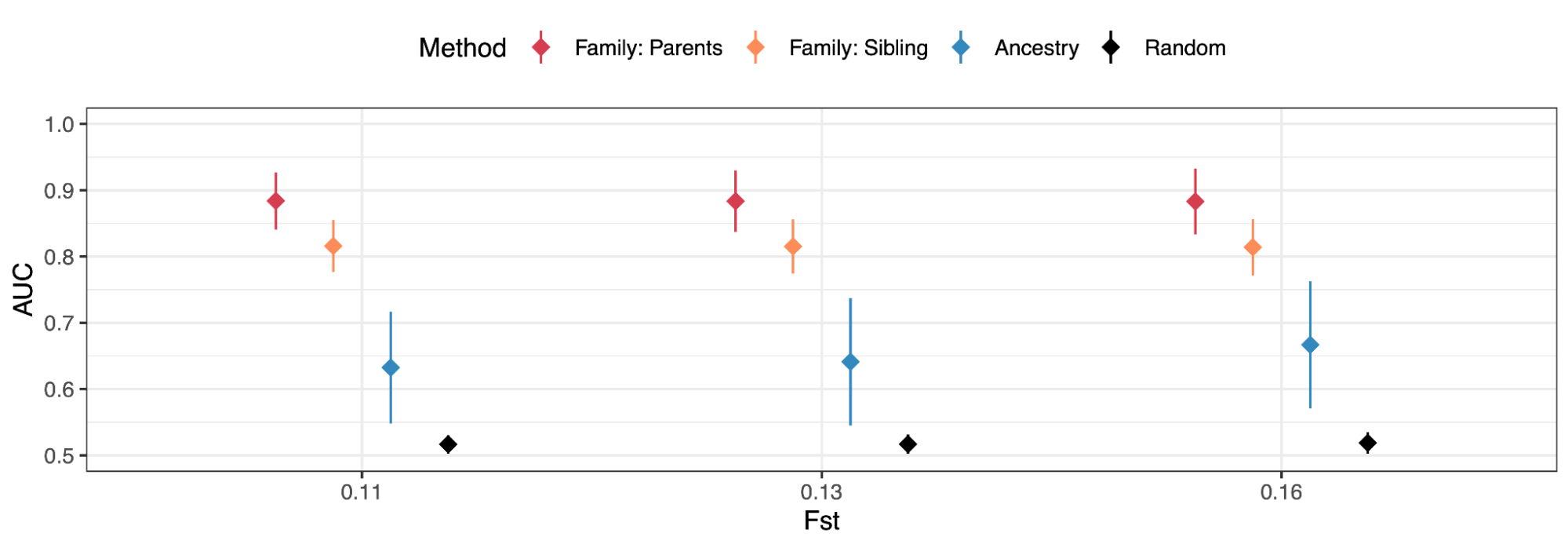
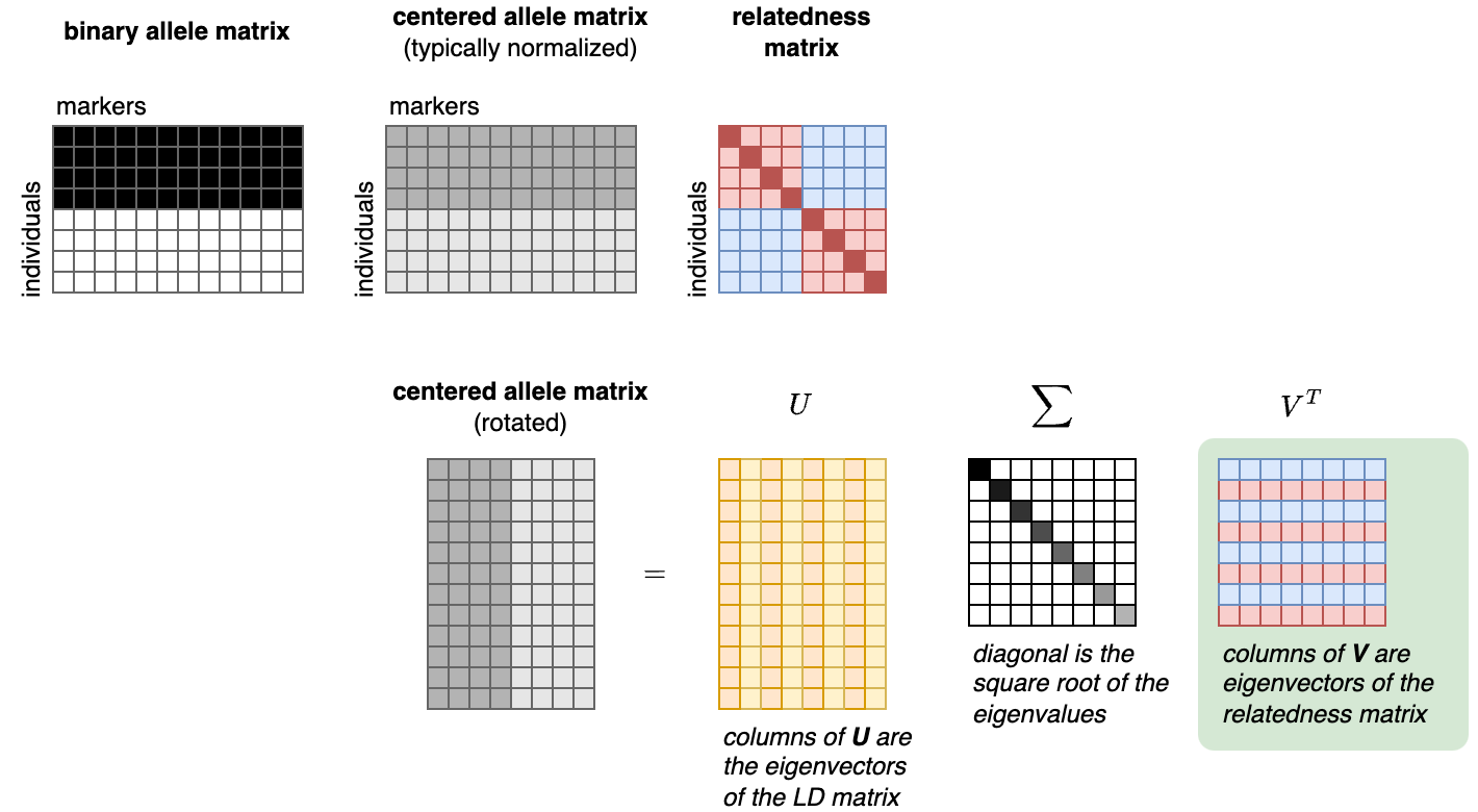
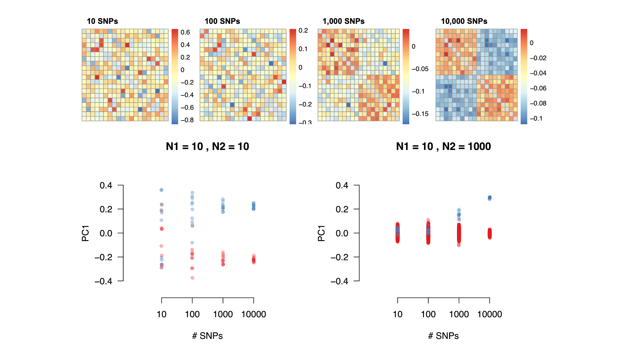
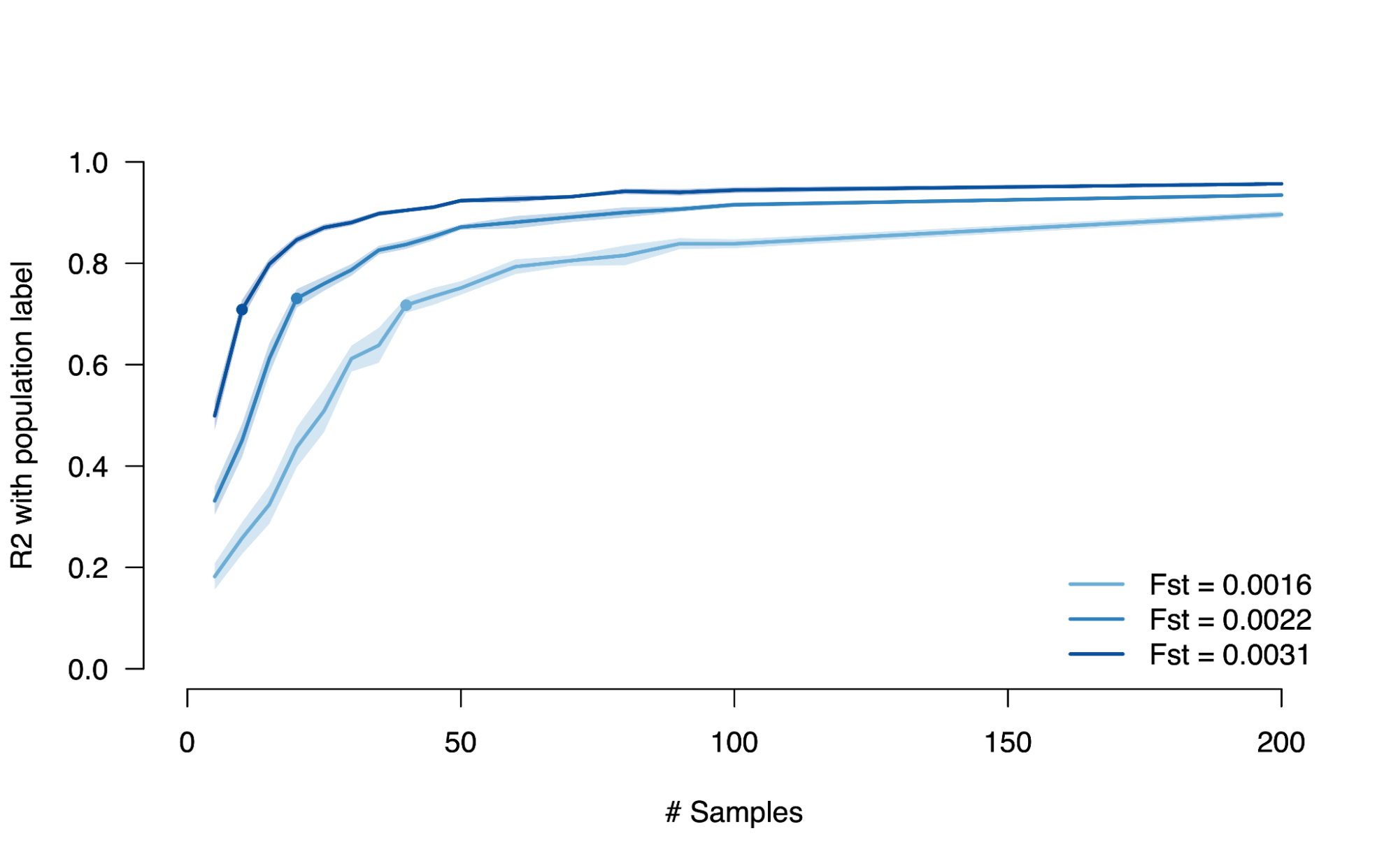
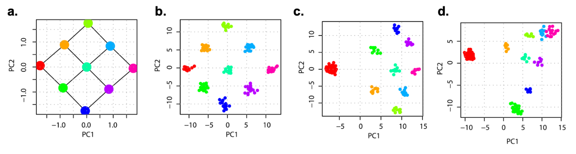
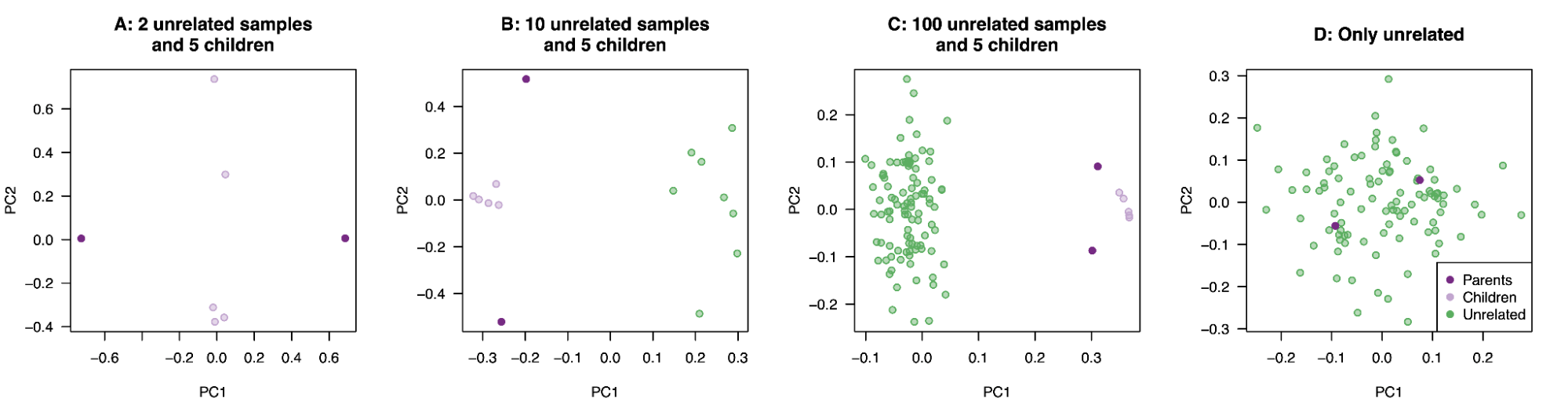
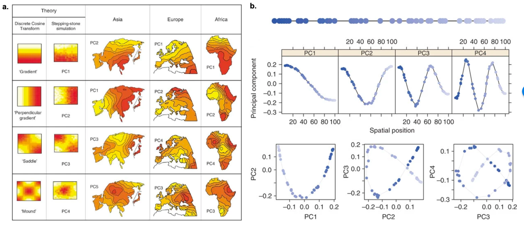
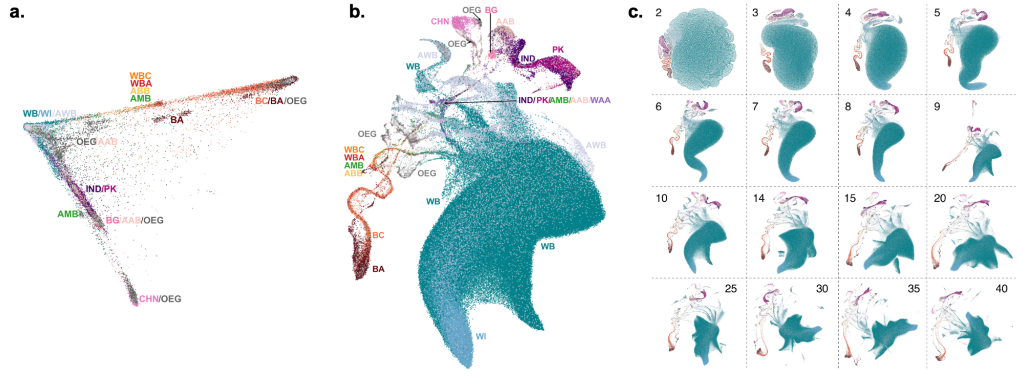
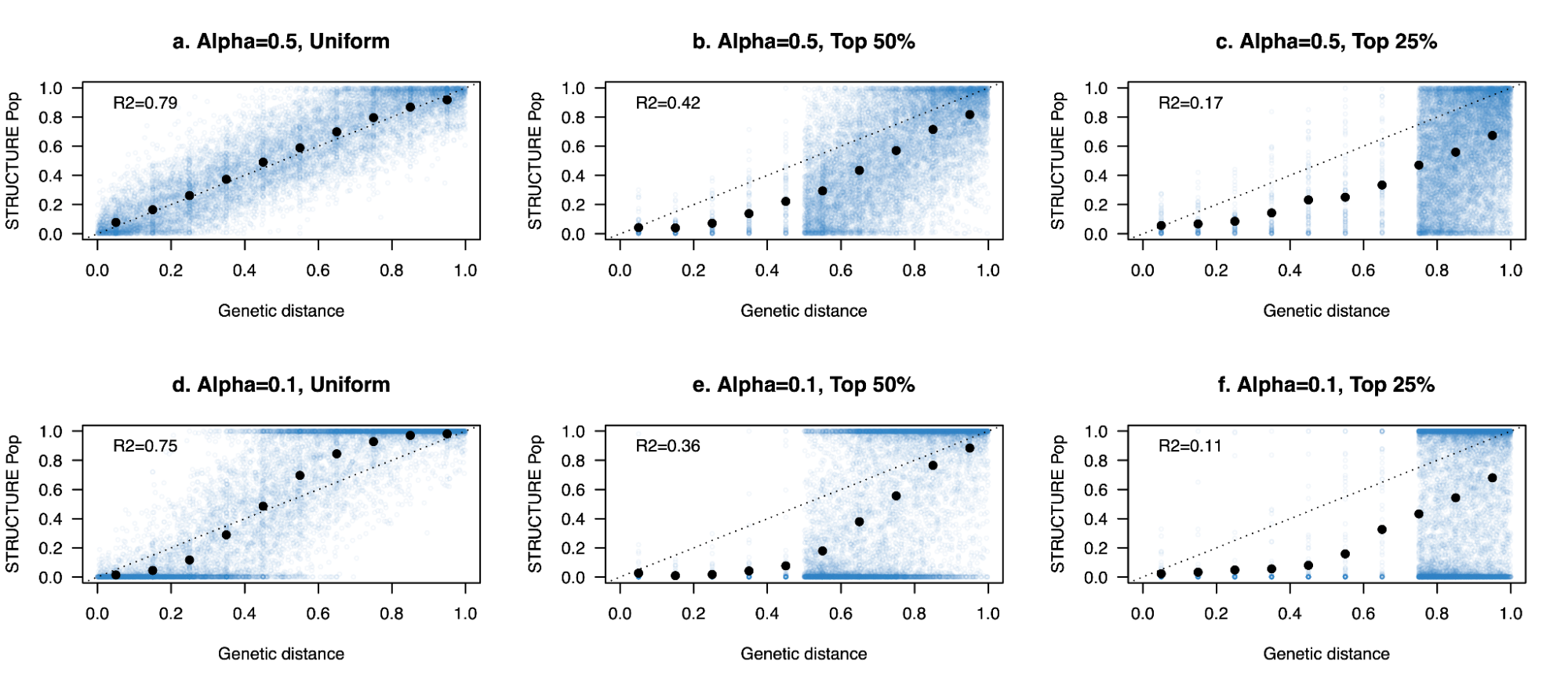
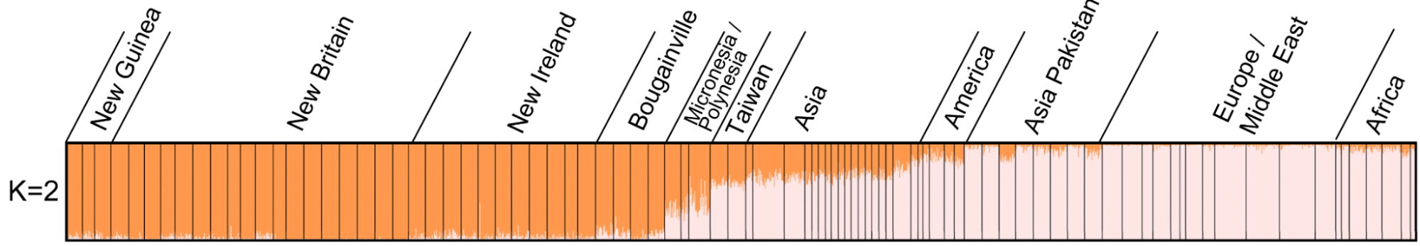
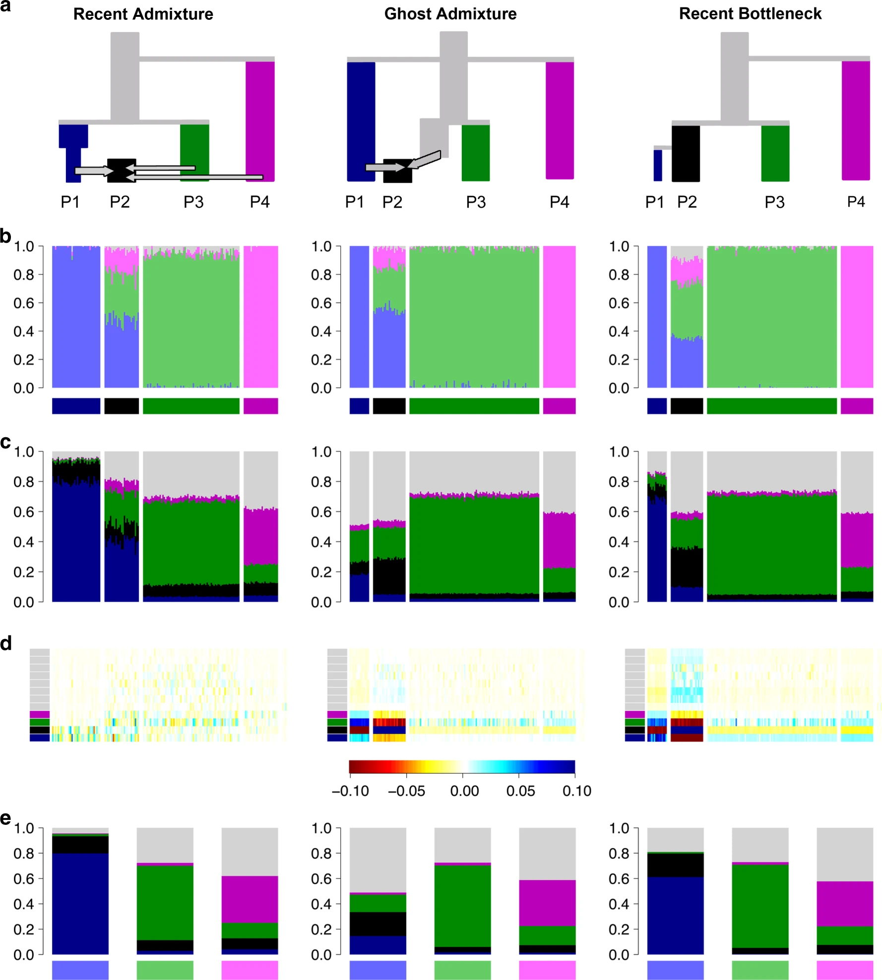
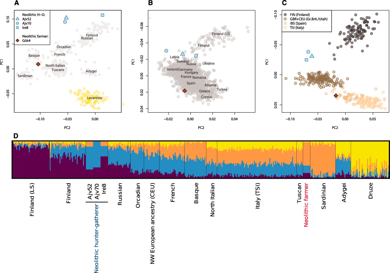
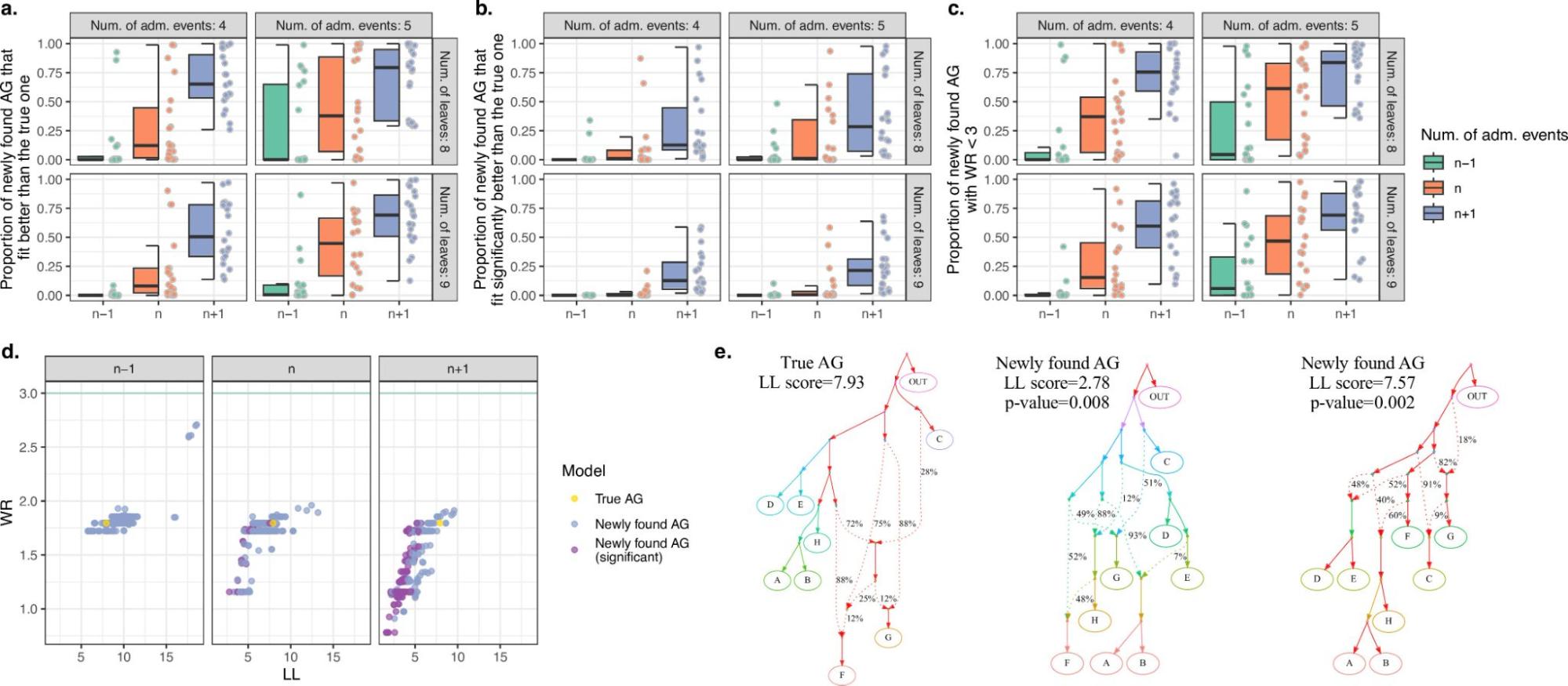
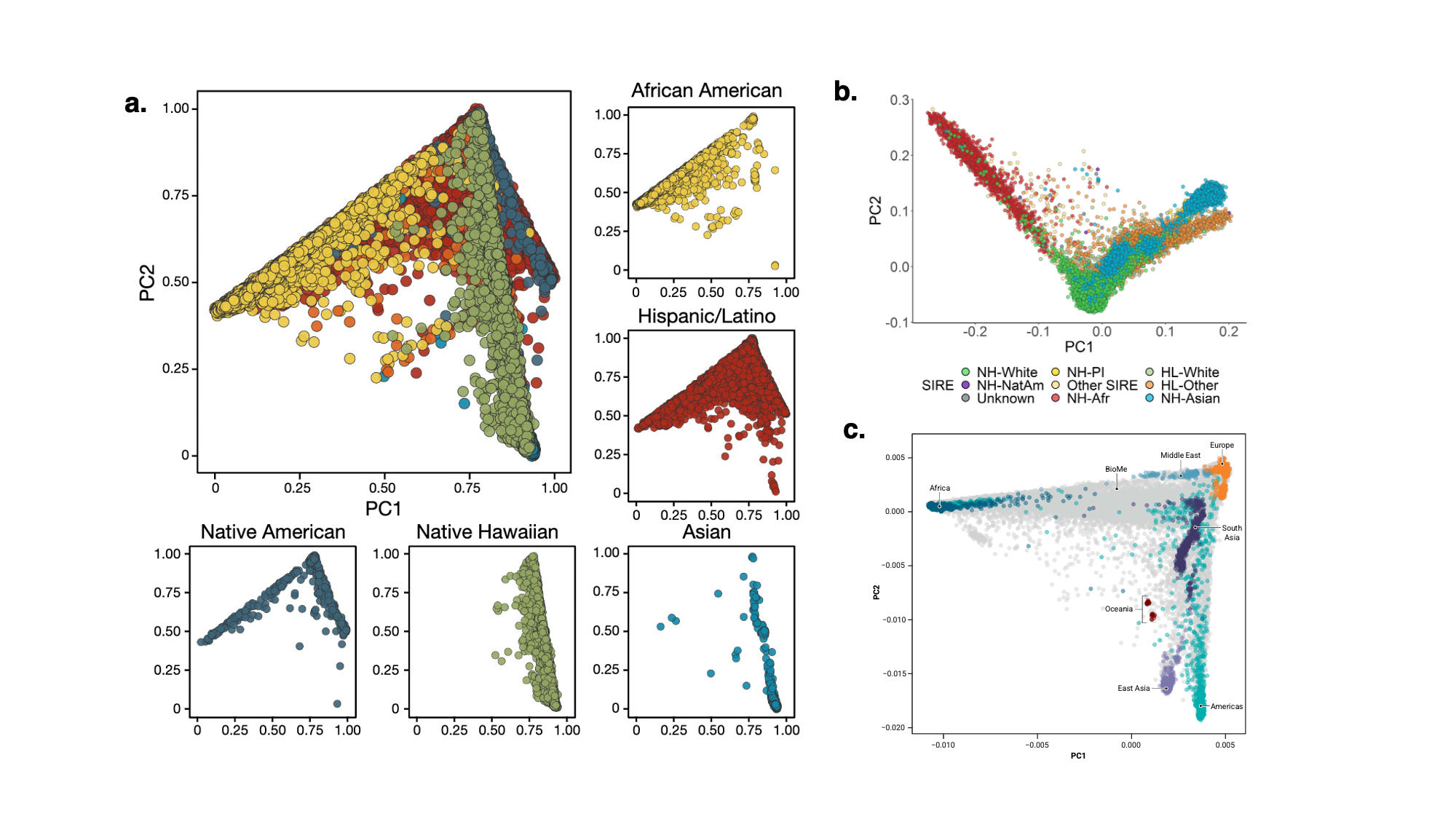
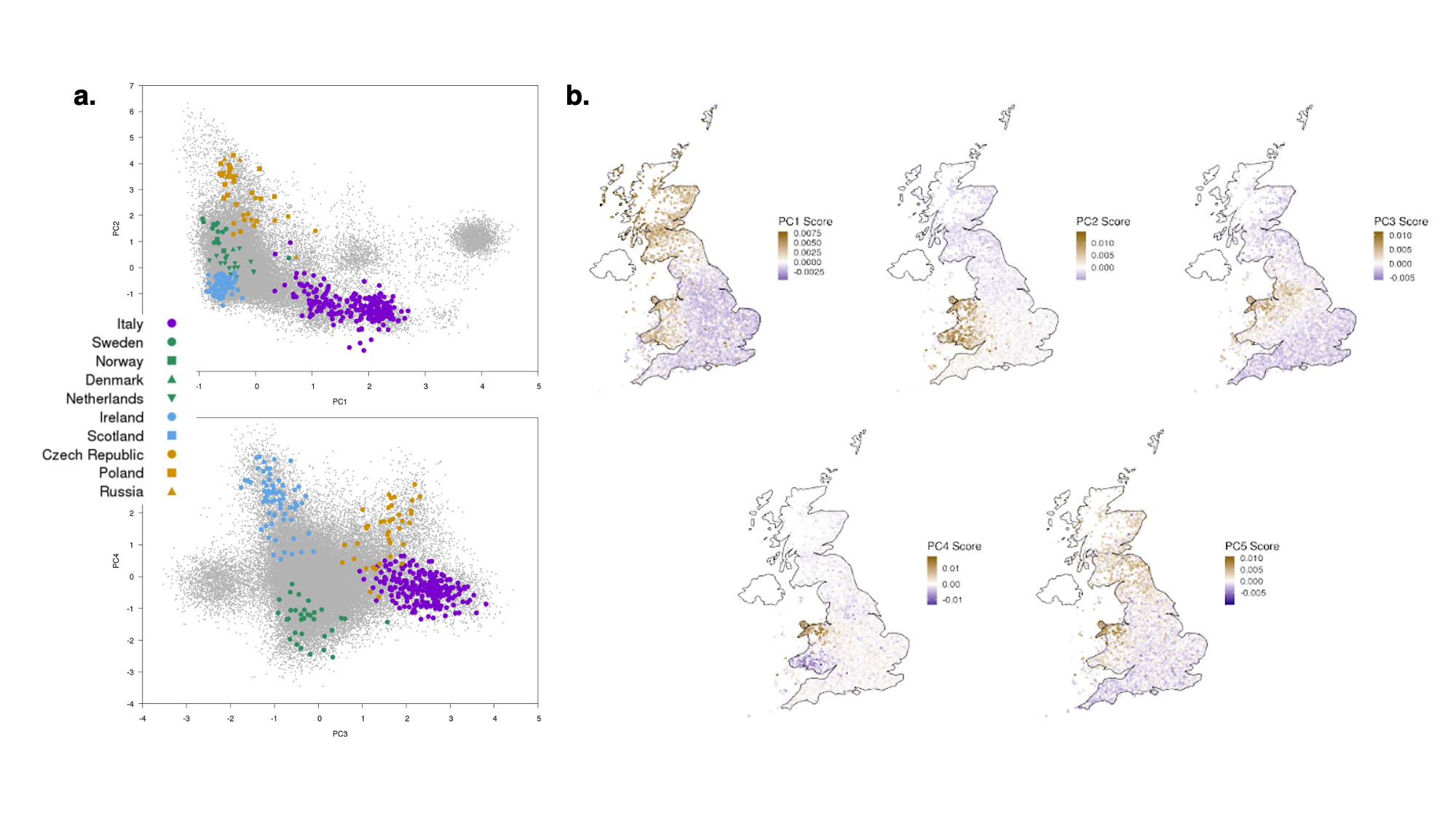
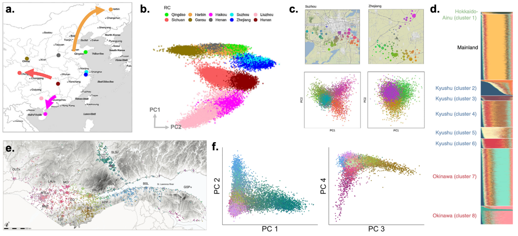
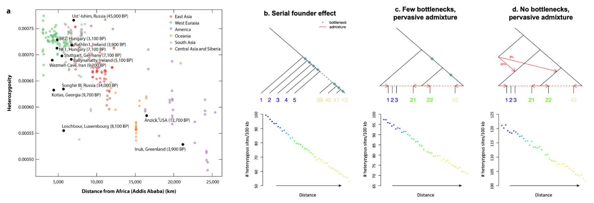
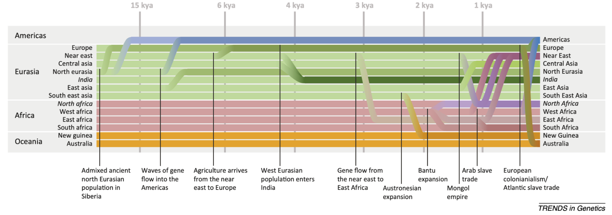
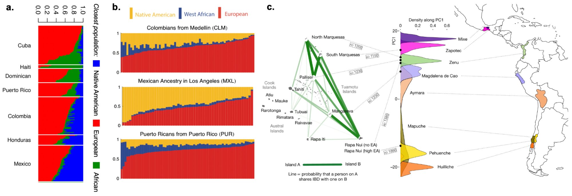
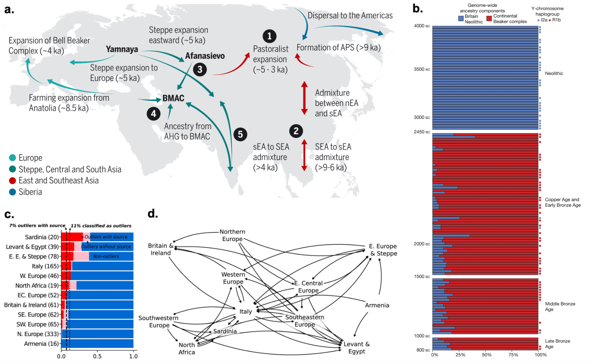
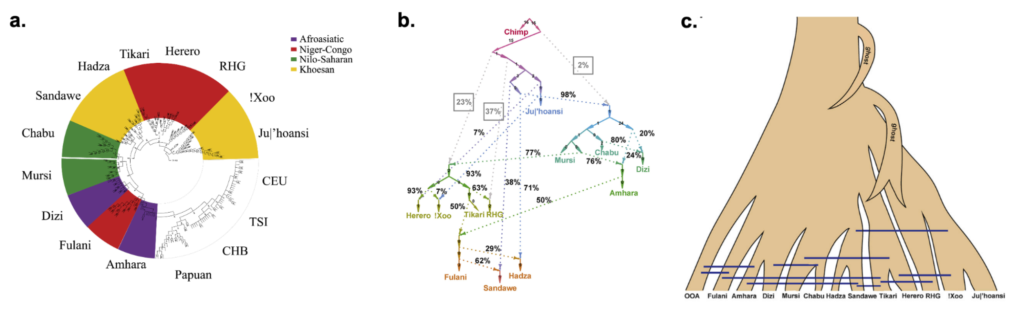
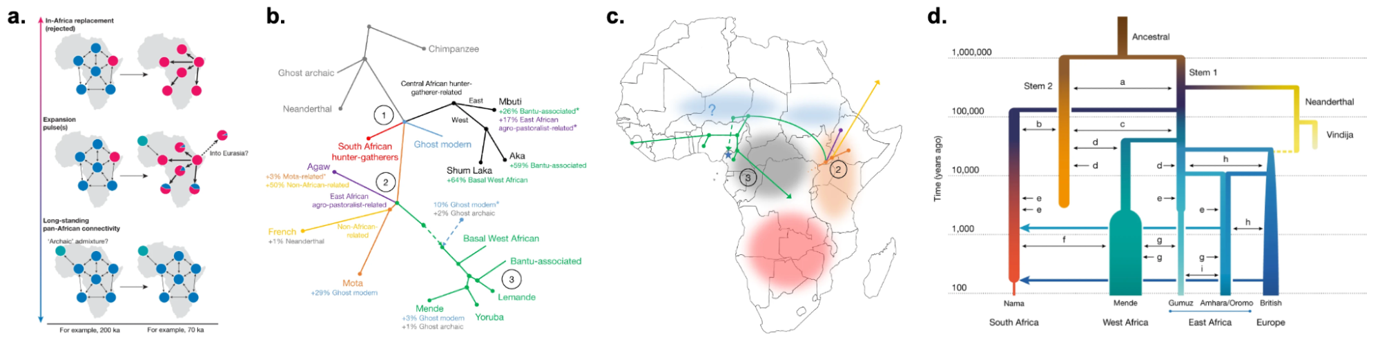